Testing for randomness

Thus, it is important to realize that even the ``random'' samples are deterministic. They are designed to optimize performance on statistical tests. Many sophisticated statistical tests of uniform randomness are used. One of the simplest, the chi-square test, is described here. This test measures how far computed statistics are from their expected value. As a simple example, suppose ${\cal C}= [0,1]^2$ and is partitioned into a $10$ by $10$ array of $100$ square boxes. If a set $P$ of $k$ samples is chosen at random, then intuitively each box should receive roughly $k/100$ of the samples. An error function can be defined to measure how far from true this intuition is:

$$e(P) = \sum_{i=1}^{100} (b_i - k/100)^2 ,$$ (5.18)

in which $b_i$ is the number of samples that fall into box $i$. It is shown [521] that $e(P)$ follows a chi-squared distribution. A surprising fact is that the goal is not to minimize $e(P)$. If the error is too small, we would declare that the samples are too uniform to be random! Imagine $k = 1,000,000$ and exactly $10,000$ samples appear in each of the $100$ boxes. This yields $e(P) = 0$, but how likely is this to ever occur? The error must generally be larger (it appears in many statistical tables) to account for the irregularity due to randomness.

Figure 5.3: Irregularity in a collection of (pseudo)random samples can be nicely observed with Voronoi diagrams.

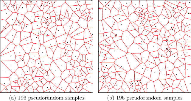
This irregularity can be observed in terms of Voronoi diagrams, as shown in Figure 5.3. The Voronoi diagram partitions ${\mathbb{R}}^2$ into regions based on the samples. Each sample $x$ has an associated Voronoi region $\operatorname{Vor}(x)$. For any point $y \in \operatorname{Vor}(x)$, $x$ is the closest sample to $y$ using Euclidean distance. The different sizes and shapes of these regions give some indication of the required irregularity of random sampling. This irregularity may be undesirable for sampling-based motion planning and is somewhat repaired by the deterministic sampling methods of Sections 5.2.3 and 5.2.4 (however, these methods also have drawbacks).