Next: 5.3 Collision Detection Up: 5.2.4 Low-Discrepancy Sampling Previous: Relating dispersion and discrepancy
Due to the fundamental importance of numerical integration and the intricate link between discrepancy and integration error, most sampling literature has led to low-discrepancy sequences and point sets [738,893,937]. Although motion planning is quite different from integration, it is worth evaluating these carefully constructed and well-analyzed samples. Their potential use in motion planning is no less reasonable than using pseudorandom sequences, which were also designed with a different intention in mind (satisfying statistical tests of randomness).
Low-discrepancy sampling methods can be divided into three categories:
1) Halton/Hammersley sampling; 2) (t,s)-sequences and (t,m,s)-nets;
and 3) lattices. The first category represents one of the earliest
methods, and is based on extending the van der Corput sequence.
The Halton sequence is an ![]() -dimensional generalization of the
van der Corput sequence, but instead of using binary representations,
a different basis is used for each coordinate [430]. The
result is a reasonable deterministic replacement for random samples in
many applications. The resulting discrepancy (and dispersion) is
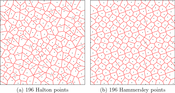
lower than that for random samples (with high probability). Figure
5.8a shows the first
-dimensional generalization of the
van der Corput sequence, but instead of using binary representations,
a different basis is used for each coordinate [430]. The
result is a reasonable deterministic replacement for random samples in
many applications. The resulting discrepancy (and dispersion) is
lower than that for random samples (with high probability). Figure
5.8a shows the first ![]() Halton points in
Halton points in
![]() .
.
Choose ![]() relatively prime integers
relatively prime integers
![]() (usually the first
(usually the first ![]() primes,
primes, ![]() ,
, ![]() ,
, ![]() , are
chosen). To construct the
, are
chosen). To construct the ![]() th sample, consider the base-
th sample, consider the base-![]() representation for
representation for ![]() , which takes the form
, which takes the form
![]() . The following point in
. The following point in ![]() is obtained by
reversing the order of the bits and moving the decimal point (as was
done in Figure 5.2):
is obtained by
reversing the order of the bits and moving the decimal point (as was
done in Figure 5.2):
 |
(5.24) |
| (5.25) |
Suppose instead that ![]() , the required number of points, is known. In
this case, a better distribution of samples can be obtained. The
Hammersley point set [431] is an adaptation of the Halton
sequence. Using only
, the required number of points, is known. In
this case, a better distribution of samples can be obtained. The
Hammersley point set [431] is an adaptation of the Halton
sequence. Using only ![]() distinct primes and starting at
distinct primes and starting at ![]() ,
the
,
the ![]() th sample in a Hammersley point set with
th sample in a Hammersley point set with ![]() elements is
elements is
| (5.26) |
The construction of Halton/Hammersley samples is simple and efficient, which has led to widespread application. They both achieve asymptotically optimal discrepancy; however, the constant in their asymptotic analysis increases more than exponentially with dimension [738]. The constant for the dispersion also increases exponentially, which is much worse than for the methods of Section 5.2.3.
 |
Improved constants are obtained for sequences and finite points by
using (t,s)-sequences, and (t,m,s)-nets, respectively
[738]. The key idea is to enforce zero discrepancy over
particular subsets of
![]() known as canonical rectangles, and
all remaining ranges in
known as canonical rectangles, and
all remaining ranges in
![]() will contribute small amounts to
discrepancy. The most famous and widely used (t,s)-sequences are
Sobol' and Faure (see
[738]). The Niederreiter-Xing
(t,s)-sequence has the best-known
asymptotic constant,
will contribute small amounts to
discrepancy. The most famous and widely used (t,s)-sequences are
Sobol' and Faure (see
[738]). The Niederreiter-Xing
(t,s)-sequence has the best-known
asymptotic constant, ![]() , in which
, in which ![]() is a small positive
constant [739].
is a small positive
constant [739].
The third category is lattices, which can be
considered as a generalization of grids that allows nonorthogonal axes
[682,893,959]. As an example, consider Figure
5.5b, which shows ![]() lattice points generated by the
following technique. Let
lattice points generated by the
following technique. Let ![]() be a positive irrational number.
For a fixed
be a positive irrational number.
For a fixed ![]() , generate the
, generate the ![]() th point according to
th point according to
![]() , in which
, in which ![]() denotes the fractional part of the
real value (modulo-one arithmetic). In Figure 5.5b,
denotes the fractional part of the
real value (modulo-one arithmetic). In Figure 5.5b,
![]() , the golden
ratio. This procedure can be generalized to
, the golden
ratio. This procedure can be generalized to ![]() dimensions by picking
dimensions by picking ![]() distinct irrational numbers. A technique
for choosing the
distinct irrational numbers. A technique
for choosing the ![]() parameters by using the roots of irreducible
polynomials is discussed in [682]. The
parameters by using the roots of irreducible
polynomials is discussed in [682]. The ![]() th sample in the
lattice is
th sample in the
lattice is
 |
(5.27) |
Recent analysis shows that some lattice sets achieve asymptotic
discrepancy that is very close to that of the best-known nonlattice
sample sets [445,938]. Thus, restricting the points to lie
on a lattice seems to entail little or no loss in performance, but
has the added benefit of a regular neighborhood structure that is
useful for path planning. Historically, lattices have required the
specification of ![]() in advance; however, there has been increasing
interest in extensible lattices, which are infinite sequences
[446,938].
in advance; however, there has been increasing
interest in extensible lattices, which are infinite sequences
[446,938].
Steven M LaValle 2012-04-20