Next: 6.3 Cell Decompositions Up: 6.2 Polygonal Obstacle Regions Previous: 6.2.3 Maximum-Clearance Roadmaps
Instead of generating paths that maximize clearance, suppose that the
goal is to find shortest paths. This leads to the shortest-path
roadmap, which is also called the reduced visibility graph in
[588]. The idea was first introduced in [742] and may
perhaps be the first example of a motion planning algorithm. The
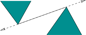
shortest-path roadmap is in direct conflict with maximum clearance
because shortest paths tend to graze the corners of
![]() . In fact,
the problem is ill posed because
. In fact,
the problem is ill posed because
![]() is an open set. For any
path
is an open set. For any
path
![]() , it is always possible to find a
shorter one. For this reason, we must consider the problem of
determining shortest paths in
, it is always possible to find a
shorter one. For this reason, we must consider the problem of
determining shortest paths in
![]() , the closure of
, the closure of
![]() . This means that the robot is allowed to ``touch'' or
``graze'' the obstacles, but it is not allowed to penetrate them. To
actually use the computed paths as solutions to a motion planning
problem, they need to be slightly adjusted so that they come very
close to
. This means that the robot is allowed to ``touch'' or
``graze'' the obstacles, but it is not allowed to penetrate them. To
actually use the computed paths as solutions to a motion planning
problem, they need to be slightly adjusted so that they come very
close to
![]() but do not make contact. This slightly increases
the path length, but the additional cost can be made arbitrarily small
as the path gets arbitrarily close to
but do not make contact. This slightly increases
the path length, but the additional cost can be made arbitrarily small
as the path gets arbitrarily close to
![]() .
.
 |
 |
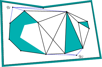 |
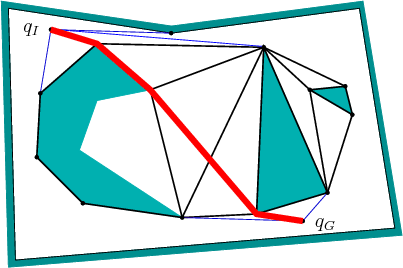
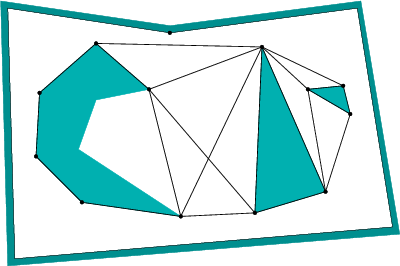
The shortest-path roadmap, ![]() , is constructed as follows.
Let a reflex vertex be a polygon vertex for which the interior
angle (in
, is constructed as follows.
Let a reflex vertex be a polygon vertex for which the interior
angle (in
![]() ) is greater than
) is greater than ![]() . All vertices of a convex
polygon (assuming that no three consecutive vertices are collinear)
are reflex vertices. The vertices of
. All vertices of a convex
polygon (assuming that no three consecutive vertices are collinear)
are reflex vertices. The vertices of ![]() are the reflex
vertices. Edges of
are the reflex
vertices. Edges of ![]() are formed from two different sources:
are formed from two different sources:
 |
If the bitangent tests are performed naively, then the resulting
algorithm requires ![]() time, in which
time, in which ![]() is the number of
vertices of
is the number of
vertices of
![]() . There are
. There are ![]() pairs of reflex vertices that
need to be checked, and each check requires
pairs of reflex vertices that
need to be checked, and each check requires ![]() time to make
certain that no other edges prevent their mutual visibility. The
plane-sweep principle from Section 6.2.2 can be adapted to
obtain a better algorithm, which takes only
time to make
certain that no other edges prevent their mutual visibility. The
plane-sweep principle from Section 6.2.2 can be adapted to
obtain a better algorithm, which takes only
![]() time. The
idea is to perform a radial sweep from each reflex vertex,
time. The
idea is to perform a radial sweep from each reflex vertex, ![]() . A ray is
started at
. A ray is
started at
![]() , and events occur when the ray touches
vertices. A set of bitangents through
, and events occur when the ray touches
vertices. A set of bitangents through ![]() can be computed in this way
in
can be computed in this way
in
![]() time. Since there are
time. Since there are ![]() reflex vertices, the
total running time is
reflex vertices, the
total running time is
![]() . See Chapter 15 of
[264] for more details. There exists an algorithm
that can compute the shortest-path roadmap in time
. See Chapter 15 of
[264] for more details. There exists an algorithm
that can compute the shortest-path roadmap in time
![]() ,
in which
,
in which ![]() is the total number of edges in the roadmap
[384]. If the obstacle region is described by a simple
polygon, the time complexity can be reduced to
is the total number of edges in the roadmap
[384]. If the obstacle region is described by a simple
polygon, the time complexity can be reduced to ![]() ; see
[709] for many shortest-path variations and references.
; see
[709] for many shortest-path variations and references.
To improve numerical robustness, the shortest-path roadmap can be
implemented without the use of trigonometric functions. For a
sequence of three points, ![]() ,
, ![]() ,
, ![]() , define the
left-turn predicate,
, define the
left-turn predicate,
![]() TRUE
TRUE![]() FALSE
FALSE![]() , as
, as
![]() TRUE if and
only if
TRUE if and
only if ![]() is to the left of the ray that starts at
is to the left of the ray that starts at ![]() and
pierces
and
pierces ![]() . A point
. A point ![]() is a reflex vertex if and only if
is a reflex vertex if and only if
![]() TRUE, in which
TRUE, in which ![]() and
and ![]() are the points
before and after, respectively, along the boundary of
are the points
before and after, respectively, along the boundary of
![]() . The
bitangent test can be performed by assigning points as shown in Figure
6.14. Assume that no three points are collinear
and the segment that connects
. The
bitangent test can be performed by assigning points as shown in Figure
6.14. Assume that no three points are collinear
and the segment that connects ![]() and
and ![]() is not in collision. The pair,
is not in collision. The pair,
![]() ,
, ![]() , of vertices should receive a bitangent edge if the
following sentence is
FALSE:
, of vertices should receive a bitangent edge if the
following sentence is
FALSE:
| (6.1) |
 |
(6.2) |