Next: Introducing more players Up: 10.5.3 Other Sequential Games Previous: Nash equilibria in sequential
 |
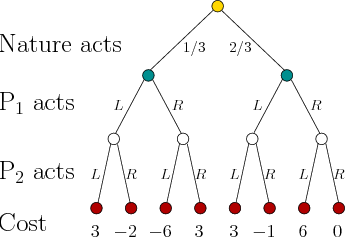
A nature player can easily be introduced into a game. Suppose, for
example, that nature is introduced into a zero-sum game. In this
case, there are three players:
![]() ,
,
![]() , and nature. Figure
10.19 shows a game tree for a single-stage, zero-sum game
that involves nature. It is assumed that all three players act at the
same time, which fits the stage-by-stage model. Many other
information models are possible. Suppose that probabilistic
uncertainty is used to model nature, and it is known that nature
chooses the left branch with probability
, and nature. Figure
10.19 shows a game tree for a single-stage, zero-sum game
that involves nature. It is assumed that all three players act at the
same time, which fits the stage-by-stage model. Many other
information models are possible. Suppose that probabilistic
uncertainty is used to model nature, and it is known that nature
chooses the left branch with probability ![]() and the right branch
with probability
and the right branch
with probability ![]() . Depending on the branch chosen by nature, it
appears that
. Depending on the branch chosen by nature, it
appears that
![]() and
and
![]() will play a specific
will play a specific
![]() matrix
game. With probability
matrix
game. With probability ![]() , the cost matrix will be
, the cost matrix will be
Several other variations are possible. If nature is modeled
nondeterministically, then a matrix of worst-case regrets can be
formed to determine whether it is possible to eliminate regret. A
sequential version of games such as the one in Figure 10.19
can be considered. In each stage, there are three substages in which
nature,
![]() , and
, and
![]() all act. The bottom-up approach from Section
10.5.1 can be applied to decompose the tree into many
single-stage games. Their costs can be propagated upward to the root
in the same way to obtain an equilibrium solution.
all act. The bottom-up approach from Section
10.5.1 can be applied to decompose the tree into many
single-stage games. Their costs can be propagated upward to the root
in the same way to obtain an equilibrium solution.
Formulation 10.4 can be easily extended to include nature in
games over state spaces. For each ![]() , a nature action set is defined
as
, a nature action set is defined
as ![]() . The state transition equation is defined as
. The state transition equation is defined as
Steven M LaValle 2012-04-20