Exercises

1. For the environment in Figure 12.1a, give the nondeterministic I-states for the action sequence $({\rm L},{\rm L},{\rm F},{\rm B},{\rm F},{\rm R},{\rm F},{\rm F})$, if the initial state is the robot in position $3$ facing north and the initial I-state is ${\eta_0}= X$.
2. Describe how to apply the algorithm from Figure 10.6 to design an information-feedback plan that takes a map of a grid and performs localization.

   Figure 12.54: An environment for grid-based localization.

   
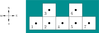
3. Suppose that a robot operates in the environment shown in Figure 12.54 using the same motion and sensing model as in Example 12.1. Design an information-feedback plan that is as simple as possible and successfully localizes the robot, regardless of its initial state. Assume the initial condition ${\eta_0}= X$.
4. Prove that the robot can use the latitude and orientation information to detect the unique point of each obstacle boundary in the maze searching algorithm of Section 12.3.1.
5. Suppose once again that a robot is placed into one of the six environments shown in Figure 12.12. It is initially in the upper right cell facing north; however, the initial condition is ${\eta_0}= X$. Determine the sequence of sensor observations and nondeterministic I-states as the robot executes the action sequence $({\rm F},{\rm R},{\rm B},{\rm F},{\rm L},{\rm L},{\rm F})$.
6. Prove that the counter in the maze searching algorithm of Section 12.3.1 can be replaced by two pebbles, and the robot can still solve the problem by simulating the counter. The robot can place either pebble on a tile, detect them when the robot is on the same tile, and can pick them up to move them to other tiles.
7. Continue the trajectory shown in Figure 12.23 until the goal is reached using the Bug2 strategy.
8. Show that the competitive ratio for the doubling spiral motion applied to the lost-cow problem of Figure 12.26 is $9$.
9. Generalize the lost-cow problem so that there are $n$ fences that emanate from the current cow location ($n=2$ for the original problem).
   1. If the cow is told that the gate is along only one unknown fence and is no more than one unit away, what is the competitive ratio of the best plan that you can think of?
   2. Suppose the cow does not know the maximum distance to the gate. Propose a plan that solves the problem and establish its competitive ratio.

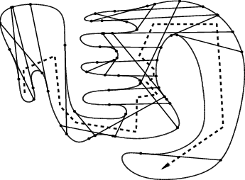
   Figure 12.55: A path followed by the robot in an initially unknown environment. The robot finishes in the lower right.

   
10. Suppose a point robot is dropped into the environment shown in Figure 12.42. Indicate the gap navigation trees that are obtained as the robot moves along the path shown in Figure 12.55.
11. Construct an example for which the worst case bound, (12.25), for Bug1 is obtained.

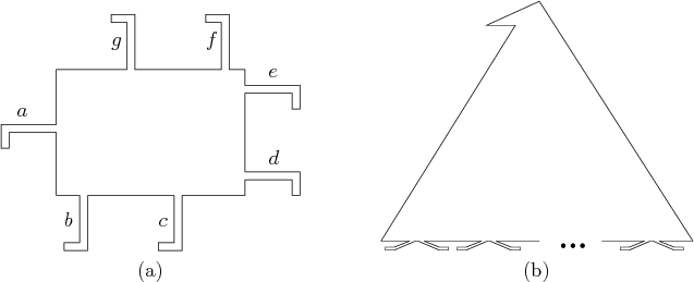
    Figure 12.56: Two pursuit-evasion problems that involve recontamination.

    
12. Some environments are so complicated that in the pursuit-evasion problem they require the same region to be visited multiple times. Find a solution for a single pursuer with omnidirectional visibility to the problem in Figure 12.56a.
13. Find a pursuit-evasion solution for a single pursuer with omnidirectional visibility to the problem in Figure 12.56b, in which any number of pairs of ``feet'' may appear on the bottom of the polygon.
14. Prove that for a polygonal environment, if there are three points, $p_1$, $p_2$, and $p_3$, for which $V(V(p_1))$, $V(V(p_2))$, and $V(V(p_3))$ are pairwise-disjoint, then the problem requires more than one pursuer.
15. Prove that the diameter function for the squeezing algorithm in Section 12.5.2 has no more than $O(n^2)$ vertices. Give a sequence of polygons that achieves this bound. What happens for a regular polygon?
16. Develop versions of (12.8) and (12.9) for state-nature sensor mappings.
17. Develop versions of (12.8) and (12.9) for history-based sensor mappings.
18. Describe in detail the I-map used for maze searching in Section 12.3.1. Indicate how this is an example of dramatically reducing the size of the I-space, as described in Section 11.2. Is a sufficient I-map obtained?
19. Describe in detail the I-map used in the Bug1 algorithm. Is a sufficient I-map obtained?
20. Suppose that several teams of point robots move around in a simple polygon. Each robot has an omnidirectional visibility sensor and would like to keep track of information for each shadow region. For each team and shadow region, it would like to record one of three possibilities: 1) There are definitely no team members in the region; 2) there may possibly be one or more; 3) there is definitely at least one.
    1. Define a nondeterministic I-space based on labeling gaps that captures the appropriate information. The I-space should be defined with respect to one robot (each will have its own).
    2. Design an algorithm that keeps track of the nondeterministic I-state as the robot moves through the environments and observes others.
21. Recall the sequence of connected corridors shown in Figure 12.40. Try to adapt the polygons so that the same number of pursuers is needed, but there are fewer polygon edges. Try to use as few edges as possible.

    
    Implementations
    

22. Solve the probabilistic passive localization problem of Section 12.2.3 for 2D grids. Implement your solution and demonstrate it on several interesting examples.
23. Implement the exact value-iteration method described in Section 12.1.3 to compute optimal cost-to-go functions. Test the implementation on several small examples. How large can you make $K$, $\Theta$, and $\Psi$?
24. Develop and implement a graph search algorithm that searches on ${\cal I}_{ndet}$ to perform robot localization on a 2D grid. Test the algorithm on several interesting examples. Try developing search heuristics that improve the performance.
25. Implement the Bug1, Bug2, and VisBug (with unlimited radius) algorithms. Design a good set of examples for illustrating their relative strengths and weaknesses.
26. Implement software that computes probabilistic I-states for localization as the robot moves in a grid.
27. Implement the method of Section 12.3.4 for simply connected environments and demonstrate it in simulation for polygonal environments.
28. Implement the pursuit-evasion algorithm for a single pursuer in a simple polygon.
29. Implement the part-squeezing algorithm presented in Section 12.5.2.