Next: 13.4.1.2 Hamilton's principle of Up: 13.4.1 Lagrangian Mechanics Previous: 13.4.1 Lagrangian Mechanics
Lagrangian mechanics is based on the calculus of variations,
which is the subject of optimization over a space of paths. One of
the most famous variational problems involves constraining a particle
to travel along a curve (imagine that the particle slides along a
frictionless track). The problem is to find the curve for which the
ball travels from one point to the other, starting at rest, and being
accelerated only by gravity. The solution is a cycloid function called the Brachistochrone curve
[841]. Before this problem is described further, recall the
classical optimization problem from calculus in which the task is to
find extremal values (minima and maxima) of a function. Let
![]() denote a smooth function from
denote a smooth function from
![]() to
to
![]() , and let
, and let ![]() denote
its value for any
denote
its value for any
![]() . From standard calculus, the extremal
values of
. From standard calculus, the extremal
values of
![]() are all
are all
![]() for which
for which
![]() . Suppose
that at some
. Suppose
that at some
![]() ,
,
![]() achieves a local minimum. To
serve as a local minimum, tiny perturbations of
achieves a local minimum. To
serve as a local minimum, tiny perturbations of ![]() should result in
larger function values. Thus, there exists some
should result in
larger function values. Thus, there exists some ![]() such that
such that
![]() for any
for any
![]() . Each
. Each
![]() represents a possible perturbation of
represents a possible perturbation of ![]() .
.
The calculus of variations addresses a harder problem in which
optimization occurs over a space of functions. For each function, a
value is assigned by a criterion called a
functional.13.10 A procedure analogous to taking the derivative
of the function and setting it to zero will be performed. This will
be arrived at by considering tiny perturbations of an entire function,
as opposed to the ![]() perturbations mentioned above. Each
perturbation is itself a function, which is called a variation. For a function to minimize
a functional, any small enough perturbation of it must yield a larger
functional value. In the case of optimizing a function of one
variable, there are only two directions for the perturbation:
perturbations mentioned above. Each
perturbation is itself a function, which is called a variation. For a function to minimize
a functional, any small enough perturbation of it must yield a larger
functional value. In the case of optimizing a function of one
variable, there are only two directions for the perturbation:
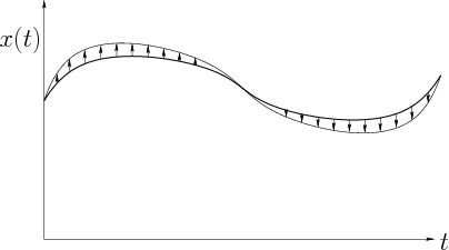
![]() . See Figure 13.12. In the calculus of
variations, there are many different ``directions'' because of the
uncountably infinite number of ways to construct a small variation
function that perturbs the original function (the set of all
variations is an infinite-dimensional function space; recall
Example 8.5).
. See Figure 13.12. In the calculus of
variations, there are many different ``directions'' because of the
uncountably infinite number of ways to construct a small variation
function that perturbs the original function (the set of all
variations is an infinite-dimensional function space; recall
Example 8.5).
Let
![]() denote a smooth function from
denote a smooth function from
![]() into
into
![]() .
The functional is defined by integrating a function over the domain of
.
The functional is defined by integrating a function over the domain of
![]() . Let
. Let ![]() be a smooth, real-valued function of three
variables,
be a smooth, real-valued function of three
variables, ![]() ,
, ![]() , and
, and ![]() .13.11 The arguments of
.13.11 The arguments of ![]() may be any
may be any
![]() and
and ![]() to yield
to yield ![]() , but each has a special
interpretation. For some smooth function
, but each has a special
interpretation. For some smooth function
![]() ,
, ![]() is used to
evaluate it at a particular
is used to
evaluate it at a particular ![]() to obtain
to obtain
![]() . A
functional
. A
functional ![]() is constructed using
is constructed using ![]() to evaluate the
whole function
to evaluate the
whole function
![]() as
as
| (13.115) |
Let ![]() be a smooth function over
be a smooth function over ![]() , and let
, and let
![]() be a
small constant. Consider the function defined as
be a
small constant. Consider the function defined as
![]() for all
for all
![]() . If
. If
![]() , then
(13.114) remains the same. As
, then
(13.114) remains the same. As ![]() is
increased or decreased, then
is
increased or decreased, then
![]() may change.
The function
may change.
The function ![]() is like the ``direction'' in a directional
derivative. If for any smooth function
is like the ``direction'' in a directional
derivative. If for any smooth function ![]() , their exists some
, their exists some
![]() such that the value
such that the value
![]() increases, then
increases, then
![]() is called an extremal of
is called an extremal of ![]() . Any small perturbation to
. Any small perturbation to
![]() causes the
value of
causes the
value of ![]() to increase. Therefore,
to increase. Therefore,
![]() behaves like a local
minimum in a standard optimization problem.
behaves like a local
minimum in a standard optimization problem.
Let
![]() for some
for some
![]() and function
and function ![]() . The
differential of a functional can be approximated as [39]
. The
differential of a functional can be approximated as [39]
 |
(13.117) |
The partial derivatives of ![]() with respect to
with respect to ![]() and
and ![]() are
defined using standard calculus. The derivative
are
defined using standard calculus. The derivative
![]() is evaluated by treating
is evaluated by treating ![]() as an ordinary variable (i.e.,
as
as an ordinary variable (i.e.,
as
![]() when the variables are named as in
when the variables are named as in
![]() ). Following this, the derivative of
). Following this, the derivative of
![]() with respect to
with respect to ![]() is taken. To illustrate this process,
consider the following example.
is taken. To illustrate this process,
consider the following example.
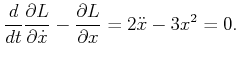
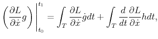
| (13.119) |
 |
(13.120) |
 |
(13.122) |