Project Description :

Problem Statement:

This project explores the problem of motion planning in a flow field.  A point mass submarine is placed in a makeshift underwater world with obstacles. The information about the world is already known, namely the position and dimensions of the obstacles, the boundaries of the world, as well as the flow field that has been precomputed using CFD Analysis.

The configuration space for the problem is R3. However, the path planning implementation is in the state space which is R6. The state space variables are x,y,and z-positions and the x,y and z velocities.

The robot running the submarine, needs to compute a path from a chosen start point to within a destination zone.  There are six thrusters on the submarine, each of which moves it in a different direction(+ve  x, y and z, and -ve x, y and z). The force provided by the thrusters is fixed (constant). The thrusters can also be used in combinations of two or three. A default option exists, not to fire any of the thrusters, if the action of the flow field is, by itself, enough to carry the submarine in the direction where it wants to go.

The robot must calculate its path, taking into consideration the obstacles(collision detection), and the constraints, of being able to fire only  one, two, or three thrusters at a time. Also the action of the flow field should also be taken into account, as the flow could either retard or accelerate the motion of the sub, or, in regions of zero velocity, have no effect.

The interaction with this application as well as the visualization of the the motion of the submarine along the calculated path will be in the C2 virtual environment.
 

Methodology

The basic path planning strategy used, is the Rapidly Exploring Random Tree (LaValle) or RRT (1).The collision detection algorithm utilised here is the simple bounding box method. Since the obstacles provided here are cuboidal, this method suffices. In more complex cases, the bitmap method is recommended.

The flow field is generated using the FLUENT CFD software and is converted to PLOT3D data format. The data is read in as a structured grid of points (71 x 17 x 31). The Visualization Toolkit software is used to read in the grid.

The algorithm is given a start state (x_init, y_init,z_init,vx_init,vy_init,vz_init,), and a goal state (x_goal, y_goal,z_goal,vx_goal, vy_goal,vz_goal).  The Random Tree starts off at the initial state,  proceeds to choose the random point and expand the tree, (for details see the link on RRT). As mentioned earlier the submarine has six thrusters, that can be fired in combinations of one, two, three or none at all. The decision on which thruster to fire is done by computing the  state of the submarine as a result of firing the thruster , and then calculating the distance from the random point chosen by the RRT. The distance metric used here is the Euclidean metric.
This can be applied in two ways a) across the 3D distance and checks which combination brings the sub closest to the random point or b)across the 6D state space and calculates the thruster combination that brings the sub closest to the random state. This point is checked for collision and if it passes the collision test (namely, it does'nt  collide), its position and velocity are then chosen as the contents of the next node and are appended to the tree. This goes on until the tree reaches a point that is closest to the goal state, or until a prespecified maximum number of nodes is added to the graph.

Dynamics:

When a goal point is picked, the RRT scans all the nodes to find the closest point. Then the dynamics of the system have to be applied in the case of each thruster, to calculate the final position of the point mass(sub).

Let the closest point be denoted by  x_curr, where x is a 6D vector containing position and velocity.
Let C be a 3D vector containg the force components of the thrusters, VF contain the fluid velocity components at the point, and a_fin be the final acceleration vector.

We then have  a_fin  =  C/m + Cd*VF/m  -- (Eq 1.), where m is the mass (1.0) and Cd is the local drag coefficient. This is calculated as the 1/sqrt(Re), where Re is the Reynolds number. For further details see (2).

Eq. 1 is integrated to give the velocity vector v_fin, which is integrated again to give the final position p_fin . Integration is done using the classic fourth-order Runge-Kutta integration. The components of v_fin and p_fin go into the state space vector for the new node.
 
 

The default action used is to set all thrusters to the off state and then compute the poistion based purely on the flow, If the flow takes the poistion closer to the random point than the current distance of the random point from the closest point, then no other thruster is fired and the sub is carried with the flow.

Once the tree is built, the closest point to the destination point is found, and the path is traced back along the tree to the initial starting position.
 

Effectiveness:

Since the RRT method is only probabilistically complete (especially after the dynamics and collision checks are implemented), we will see that there are situations where the RRT will fail to converge to within the specified distance to the goal state even after a large number of nodes have been explored. Since the RRT has to go over all the nodes every time a new random point is picked, the computation time will increase with every node that is added.

Situations where the RRT will fail to converge are

1) Where the start or destination position are placed too close to an obstacle. In this case there are two possibilities of failure
 
    a) The destination point cannot be reached easily without collision irrespective of where the randomly chosen point lies.
    b) There are vortices formed near the obstacles, which prevent the point mass from moving across them to reach the destination point. In other words, the thruster combinations would not be able to overcome the flow, and will hence be offset by the flow to different positions away from the destination.

2) The destination point lies in the middle of a vortex, which will cause the same effect as b)

3) The number of nodes are too small, or the incremental distance is too small, or the integration step size, is either too large or too small. The interaction mechanisms provided in the application, will help overcome this problem.
 
4) The source point is in a space where there are too many collisions.
 
 

Computed Examples

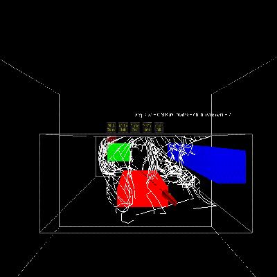
Snapshots of the application
 

 

Animated examples:

( Hit the reload button on browser to replay the animation. The animation has been  put in slow motion to allow a (hopefully) clearer visualization of the movement of the submarine and the thruster configurations )

Case 1: A simple case (Goal bias 20 %)
Here the start and destination point are in the open, unobstructed by any obstacles. However, there is still the flow field to be taken into consideration. This means that the sub, cannot neccesarily go directly towards the random point picked. This is why the path is wiggly in places. However, the start and destination points lie downstream of each other, hence the sub moves with the flow from time to time, not requiring the thrusters to be fired often. The RRT picks the goal state 20% of the time.

Case 2: A case where the start and destination point are obscured by the obstacles, but convergence still occurs
 Here,  it was seen that the path did converge, although the time taken to converge was more. This could have been due to the large number of collisions that had to be overcome, due to the goal bias. Also it took a larger number of nodes to converge than for the previous case. The constraining factors here could be attributed to the vortex pockets in the vicinity downstream of the obstacle.

Case 3: A tough case. No convergence:
This case shows the start position and the goal position in totally obscured portions of the space. The region where the goal lies is in between the face of the obstacle and the exit. It was found that convergence could not occur even when the velocity constraints and fluid field were turned off(holonomic case). This is because it was not possible for the tree to reach the goal easily without colliding. It took a large number of node iterations(about 7000) to achieve convergence in the holonomic case. The velocity field in the vicinity of this region tends heavily  towards pushing the submarine in the x direction, and thereby preventing feasible motion in the y and z direction. Hence, in the non holonomic case, it was not possible to find a solution. 

Interaction

Interaction with the application is through the C2 (CAVE) Surround Screen VR device. This can be operated in simulator mode, to provide desktop interaction. However, the major interface will be inside the actual C2. The hardware used for the interaction is the wand and track glasses (mouse pad and keys in desktop mode). The software used for the interaction is the C2 libraries. OpenGL is used to perform all the rendering. The parameter adjustment, and activation of the path planning algorithms are done through a menu interfacing system. The user interactively picks a start and destination point, and then adjusts parameters like the the no. of nodes, etc, after which, the RRT generating algorithm is activated. The user can then display the tree, or path, and perform the animation of the submarine through the flow field. There are two types of animation, walk through and continous. In the former, the user can step through the animation by pressing down on the wand buttons, and in the latter, can watch the sub make its way through at a stretch.

Conclusions and Future Work

The application was demonstrated and run in the C2. Also,  experimentation was done with different cases by adjusting the different parameters to find the path that best converged.
There are several avenues for future work and improvement. Some of which are illustrated below

Performance and interaction could be improved by parallel processing.
 
The number of degrees of freedom in the application could be extended.(To model a real prototype submarine, with 6 degrees of freedom (x,y,z,yaw,pitch,roll) ).

The obstacles could be made non convex (Improved Collision Detection algorithms).

Implementation Files

Source Code:

README

Source code archive

Makefile
main.C
NHRRT.C
NHRRT.h
RRT.C
RRT.h
 

Input Data Files:

Obstacle File: This contains the number of obstacles and the starting and ending points of the bounding box for them
f001.dat,f001.grd: These are data files for the CFD data. Since they are too large, they have been compressed and stored in the archive.
 
 

References:

1. Rapidly Exploring Random Trees, Steven LaValle

2. Fundamentals of Fluid Mechanics Munson, B.F, Okiishi, T.F, Young, D.F, 2nd Ed. John Wiley and sons, Inc., NewYork, N.Y., 1994