Project Description

The problem in this project is two understand the behavior of two algorithms that is used in path planning. Path planning algorithm plays an important role in motion strategy because it is the main body of the whole program that determines how the robot should move from it's initial position to the goal position withtout hitting any obstacles and make sure the path is short. The two algorithms that I'll be comparting is:

• Random Roadmap Planning
• Rapidly Randomly Exploring Tree (RRT)

    While designing these project, one main concerned is about the collision detection algorithm. Since my main objective is to compare path planning algorithm, I will be using a collision detection algorithm that are mostly found in the LEDA library. Both path planning algorithm will be using the same collision algorithm to avoid any inconsistencies in the data.

    The algorithms will both use the same map, initial point and goal point. Most of the algorithms are program with the help of LEDA library. The LEDA library contains many useful functions but some of them are pretty slow. This is because the obstacles in my map must be convex in order for the algorithms to work and since LEDA functions take into consideration for both convex and concave objects, it will naturally take more time to calculate.

    I've implemented the algorithms in C++ classes, this is because I don't have to changed much of the underlying code like checking for collision, adding edges to graph, vertices to graph and so on. To use the class, it is done by simple create an instance with the Obstacles, Robot and border thrown in and starting using a class function call Builld_rplanner(window W) to start building the path. The path will be slowly generated on the screen.

    One challenging part I faced when implementing the algorithm is to figure out the individual sub functions in the algorithm. This is because there are times when the problem lies in the sub-function but not in the whole algorithm. And sometimes, it is hard to tell whether the sub-functions are behaving as they should behave. The only method I can find out is to slowly debug the individual sub-functions, which take out most of my time.

Randomized Path Planning

Here's the algorithm:
-------------------------------

BUILD_ROADMAP( A, O)

1.     G.init();
2.     for i = 1 to M
3.         q <- RAND_FREE_CONF(q);
4.         G.add_vertex(q);
5.         for each v in NBHD(q, G);
6.             if ((not G.same_component(q, v)) and CONNECT(q,v)) then
7.                     G.add_edge(q,v);
8.     Return G;

    In the beginning of these algorithm, I'm connecting every vertex found in NBHD to the a configuration q (which is chosen randomly in the graph). This will cause a tremendous performance loss because we only need to find a configuration v in NBHD that have the shortest path to configuration q, yet it is not the same_component and there's a clear path to connect configuration q to configuration v. The time taken using the old algorithm takes to much time therefore I changed it to:
 

5.     for each v in NBHD(q, G);
6.         if ((not G.same_component(q,v)) and CONNECT(q,v)) then
7.                 G.add_edge(q,v);
8.                 break;

The time complexity of this algorithm will be O(M(N+ K)). N is the time to find the nearest node and K is for computing CONNECT(q,v).

The problem with using these changed algorithm is that chances of having a connected path will be lower.

For example:

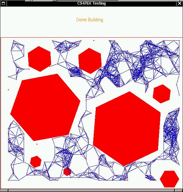
This is the graph generated with old algorithm using M with 400:

Fig 1-1 Graph using old Randomized Roadmap Algorithm

The time taken is 16 seconds.

This is the second graph generated with new_algorithm.

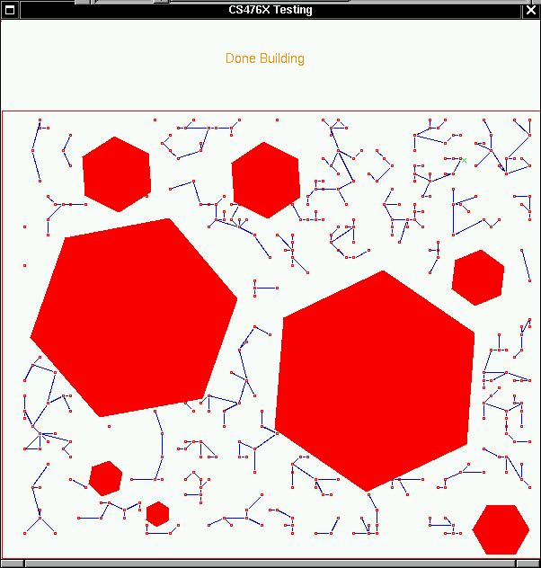
Fig 1-2 Graph using new Randomized Roadmap Algorithm

    Time taken to generate is 3 seconds, but notice in the new algorithm, the graphs are not wholly connected. You can see the individual tree not connected to the main tree. These will create a problem of finding a path. One solution of finding a path is to increase the vertices, or M in the algorithm.

    Using the same map, I tried generaing Road Map with M = { 1000, 2000, 3000} and all of them still can't find the Path from initial point to goal and time taken for M = 3000 is around 33 seconds. Therefore my conclusion is to resort back to the original algorithm.

Here's the path founded.

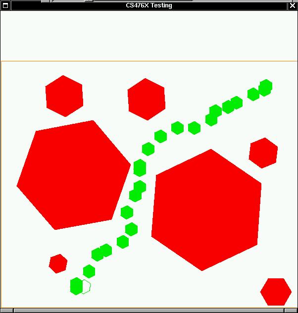
Fig 1-3 Path from Initial point to Goal point using Randomized Roadmap Algorithm.

Here's the algorithm
------------------------------

Build_RRT(A, O)

1. G.init();
2. q <- RAND_FREE_CONF();
3. G.add_vertex(q);
4. for i = 1 to M
5.     q <- RAND_FREE_CONF();
6.     v = find_nearest_node(q);
7.     q = Growth_node(q,v);
8.     if (!same_component(q,v) and connect(q,v) and infree(q) )
9.         G.add_vertex(q);
10.         G.add_edge(q, v);
11. return G;

The RRT algorithm will take be easier to implement because it didn't have the NBHD function. The find_nearest_node(q) behaves almost like NBHD but this time we don't use a proximity distance. We just get which ever node that is nearest to our random configuration. The time complexity of this algorithm will be O(M(N+ K)). N is the time to find the nearest node and K is for computing CONNECT(q,v).

Here's a sample output of the RRT generated using RRT:

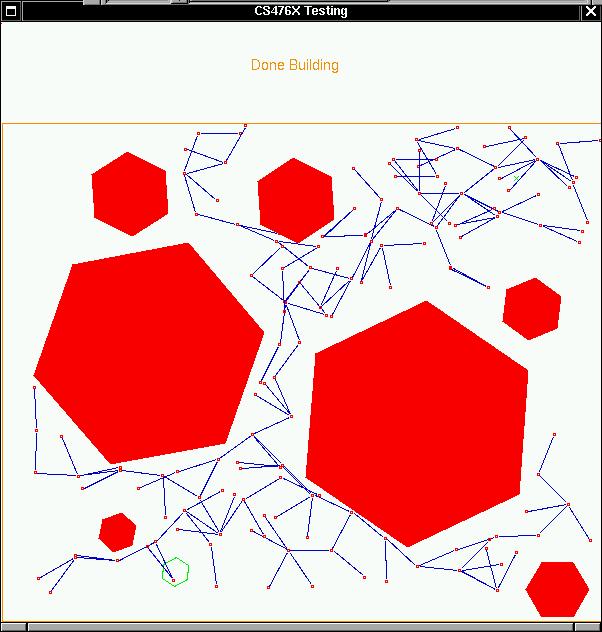
Fig 2-1 Graph using RRT
 

and this is the Path found:

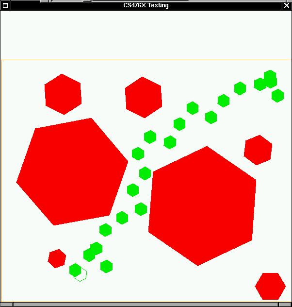
Fig 2-2 Path found using RRT

Comparison

Generating the RRT will take a lesser time than Randomized Path Planning. This is becase for the same amount of M, the RRT takes O(M(N+K)) while the RPP takes O(MNK)  less time needed. Here's a table showing the results.
 
 

M	Found-Path?		Time-Taken(seconds)
	RPP	RRT	RPP	RRT
100	No	No	1	0
200	No	Yes	4	1
300	No	Yes	8	1
400	No	Yes	16	1
500	No	Yes	23	1
600	No	Yes	34	2
700	No	Yes	47	2
800	No	Yes	60	3

Is is obvious from these table that RRT will be a better and efficient algorithm compared to RPP. But there's one disadvantage I found in RRT, and that is the path generated by RRT look weird and usually it will take longer dinstance from initial point to the goal point. For example path in fig 1-3 looks smoother and form a nice path while path in fig 2-2 looks crooked.

Implementation Files
Source Code:

• Makefile
• cs476.C
• rplaner.C
• rtplaner.C
• rplaner.h
• rtplaner.h

• test3.ascii
• test3.fig

[html] - [postscript] Notes from cs476
LEDA Manual

Instructor: Steve Lavalle