CS576 MOTION STRATEGY

PROJECT

Peng Cheng

4/2000

Path Optimalization Using Gradient Algorithm

Introduction

Long time ago, designing a robot which can replace persons to complete the work is man's dream. To realize this object, there are several key problems. One of them is motion planning problem, which is how to get the robot to move from one place to another place without hitting any obstacles.

There have been many researches on the motion planning problem since it is first pointed out in 1970's. Most of the researchers only dealed with the kinematics of the robot without considering the dynamics of robots[1][2]. But when people applied the kinematics motion planning path, they found that the path generated this way always can not be followed by robots because of the dynamic constraints of the robot. So people began to notice the motion planning problem considering both the kinematics and the dynamics, which is known as kinodynamic motion planning[3]. Kinodynamic motion planning is first pointed out in the paper of Xavier[3]. In his paper, he gave the concept of state space, used the finite set of controls to discrete the state space, and searched the discreted state space to approximate the minimal time path. While when the dimension of the state space is high, the searching time will increase very quickly. So many methods using randomized techniques have been presented. Rapidly-exploring random trees is pointed out by Lavalle[2]. The method searches the state space by extending the nearest state in the path tree, originating from the initial state, to the direction of the random state obeying the dynamic constraints. Sooner or later, when one of leaves of the tree reaches the goal state, a path is found. An application to control the autonomous vehicle using this method has gotten exiting results[4]. Probabilistic roadmap finds the path by using a two-step method. First a roadmap is generated by connecting randomly chosen state points. In the second query stage, the path can be found by just connecting the initial state and the goal state with the existing roadmap[5]. Kindel[6] successfully extended this method to find path amidst moving obstacles. Although these randomized algorithms get good results in some applications, the results are based on the loss of the optimality of the path. The random path planning algorithm avoids the rapidly increasing state space by randomly exploring the state space. So the path found is very likely to be nonoptimal, while at some situation the optimality is very important. The problem lies between the theory of control and the algorithm of computer science, so there is no related paper on this problem. The objective of this paper is to use the gradient algorithm to get some solution for this problem.

Formal problem description

The problem in this paper consists of three parts:

1. Robot, which is normally represented by a system transition function.

2. Path, which is found by using randomized algorithm and normally represented by a serial of control signals along the path.

is the time the robot begins to move, is the time the robot reaches the goal. is the control period and is a constant.

The control serial will draw the robot from the initial state, , to the goal state, with some given precision.

3. optimaliztion criteria, which is in the form as follows:

The objective of the problem is to find a path on the basis of the given path, which can make the value of as small as possible without violating the constraints of the robot.

Method

In the perspective of control theory, this problem is one of the optimal control problems. The general soution to the optimal control problem should fulfill the Hamiltonian equation[7][8] as follows:

By using these equations, we can solve many optimal problem just by some modification, such as shorting method[8], method based on Bellman’s equation[8], and the gradient algorithms[7]. The method based on Bellman’s equation has the “curse of dimensionality” problem and can not be used for high dimensional problems which are normal in the path planning problems. The shooting method should first guess an initial value for , then use the guess to compute the optimal control. Its results depend much on the guesses for . The gradient algorithm is widely used in the optimal control because it does not need the knowledge of the system. It was also used in this paper.

The gradient algorithm is given as follows:

was used to compute the state history and do the collision detection along the path. The state_history was computed by forward integrating the given system equations.

was used to compute the influence function p and R along the path according to the following equations.

At the same time some matrix integration was computed here accordintg to the following equations.

was used to compute the changes in each step of the control serial. For each step,

was used to get the new control serial from the old control serial and deltau and check whether the new control serial meets the requirement of precision for the problem. If the new control serial fulfilled the precision requirement, the new control would generate a better path than the old one.

For the path planning problem, some modification to the algorithm need to be done because the system equations for many robot are not good enough to generate the matrix with good condition number. It caused the inverse of the matrix to be inaccurate, or even impossible. This leaded to the termination of the algorithm. There were two method to deal with this problem in this paper. One was using the pseudo inverse of the matrix. It can deal with many ill condition matrix. But sometimes even the pseudo inverse was also impossible. The further method used was to check whether the pseudo inverse matrix was possible. If it was not possible, we just set for this step to be zero because we knew that the original value for this step will lead to the goal state.

In the experiments, we found that for some specific model, such as car model, the computation along the path had a lot of matrix which can not be inverted. And then there weremany 0 in the deltau. The new control computed from old control and the deltau was useless for so much 0 in the deltau. So we cut the path into many pieces, optimalized each part seperately and joined them together to get the optimalization for the whole path.

As for how to divide the path into different parts, there were two methods used in this paper. One was complete optimalization of all possible part of the path.

Complete_part_optimal

len = length of control serial

for i=2 to len

For j=1 to len-i

Gradient_algorithm(j, j+i)

The gradient_algorithm here was a little modification of original algorithm. It only optimalized the part of path from time to .

This method can find all possibly optimal part along the path. While because this method is time consuming. when the length of the control serial is a big number this method is hard to be practical.

Another method is randomized optimalization of the part of the path.

Randomized_part_optimal

len = length of control serial

For i=1 to Count

Random i, j

If (i>=1 && j<= len) gradient_algorithm(i, j)

It randomly choosed the beginning point and ending point for one part of the path and optimalized the part. When it ran a given times, it stopped and output the results. This method avoided completely search the path, but it can not gurantee to find all path parts which can be optimalized and was not easily understood so that giving a loop number was difficult.

Results

A gradient algorithm using method mentioned above was implemented in C++ on linux and Matlab.

The problem used in the experiment is as follows:

The robot was a mass point with and as pushing force. The system equation was:

The optimalization criteria was to get minimum time along the path, so the criteria function was:

The initial path was got by using Rapidly Random-exploring Tree algorithm.

The resutls was as follows:

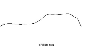
The path from RRT algorithm is showed as above. The length of the control serials for the original path was 73.

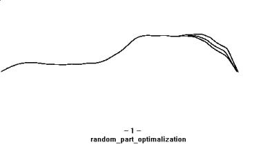
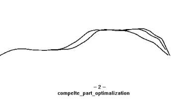
From the graph, we can see that the complete_part_optimalization got a better path than the random_part_optimalization. While according to the algorithm, the complete_part_optimalization ran local gradient algorithm for 5329 times. While the random_part_optimalization needed only 1000 times.

Conclusion

By the experiments using the optimal method given in the paper, we can see that the gradient algorithm can optimalize the path got from randomized algorithm. But there are still some further work needed. From the graph, we can see that the optimalized path had not made the criteria reach the possible minimum value. The main reason for this problem might still be the matrix with bad condition number. So further method should be developed to deal with the matrix with bad condition number.

Reference:

[1] Y. K. Hwang, N. Ahuja. Gross Motion Planning-A Survey. ACM Computing Serveys, Vol. 24, No. 3, 219-283, 1992.

[2] S. M. Lavalle, J. J.Kuffner, Jr. Randomized Kinodynamic Planning. IEEE International Conference on Robotics and Automation, 1999.

[3] P.G. Xavier. Provably-Good Approximation Algorithms for Optimal Kinodynamic Robot Motion Plans. URL=http://cs-tr.cs.cornell.edu:80/Dienst/UI/1.0/Display/ncstrl.cornell/TR92-1279, April 1992.

[4] E. Frazzoli, M.A. Dahleh, and E. Feron. Robust Hybrid Control for Autonomous Vehicle Motion Planning. December 1999.

[5] L.E. Kavraki, J. Latombe. Probabilistic Roadmaps for Robot Path Planning.

[6] R.Kindel, D.Hsu, J. Latombe, S. Rock. Kinodynamic Motion Planning Amidst Moving Obstacles. Submitted to IEEE International Conference on Robotics and Automation, 2000.

[7] E.Bryson, Jr., Yu-chi Ho. Applied Optimal Control. Hemisphere Publishing Corporation, Washington, D.C., 1975.

[8] R. Pytlak. Numerical Methods for Optimal Control, Problems with State Constraints. New York, NY, 1999.

Program:

1. model.C

2. optimal.C