Implementation With Results

  In the implementation, the input has been restricted to polygonal environments.

The first step of the algorithm is computing a cell decomposition of R. This part of the implementation requires a geometric analysis of $\partial R$, and results in a parametrized graph containing the boundary, the bitangents and the inflections. The graph contains all necessary information regarding its elements that are needed by successive modules. More or less, this includes the physical position of the elements, as well as some information on each bitangent and inflection that is needed to determine what exactly happens when the line is crossed (for example, what gap will disappear/appear).

Then a planar graph corresponding to G is constructed, with nodes placed at points where the robot is faced with a decision regarding multiple possibilities in movements, or places right before/after a pursuit event occurs. This graph can be thought of as a movement graph for the robot, where the robot can issue commands like 'go direction until a pursuit event occurs or I can choose to go in a different direction'. Notice that the movement graph induces an information state graph in which for each node of the movement graph there exist many different nodes, each corresponding to a different information state possible when the robot is located at the node of the movement graph.

To determine the edges in the information state graph, a gap tracking module had to be developed to determine how the information state changes when going between different points of the movement graph. This gap tracker takes in the gap positions and information state of the start node, and using the gap positions of the destination node and knowledge of what pursuit event occured between them determines the information state at the destination node. Although this module relies on knowledge of the map, in a real-world setting a robot would be able to determine the information state changes by simply noticing what individual gaps do through continuous movement.

A breadth first search of the information state graph is then executed, starting from some randomly chosen initial node. The search keeps going until a node with all the gaps cleared is reached, or all nodes reachable from the inital node are found to not have all gaps cleared. In the latter case, no solution for R exists. Otherwise, the search gives the sequence of nodes of the movement graph that need to be visited in order for R to be cleared.

Such a modular designed allowed the program to be developed in phases that made the programming a little easier by focusing on individual parts. However, through this modular development little attention was paid to efficient algorithms, and with all the modules put together it takes quite some time for solving complex environments. In addition, there are still bugs that cause crashes on some inputs. There is definitelly room for making a lot of the algorithms more efficient, as well as debugging the code.

In the following examples, the left image shows the cell decomposition and the right the computed solution. Red lines are inflections and green lines are bitangents. Note that the robot is moving only along green lines and the walls. All solutions were computed in under a few seconds on a 500MHz machine, except for 7 which took under a minute. Source files

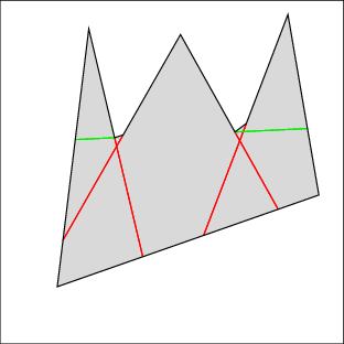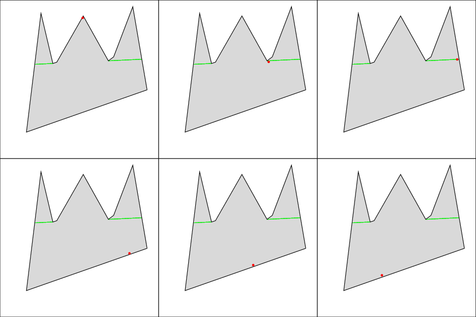Example 1: clear the right gap, then the left
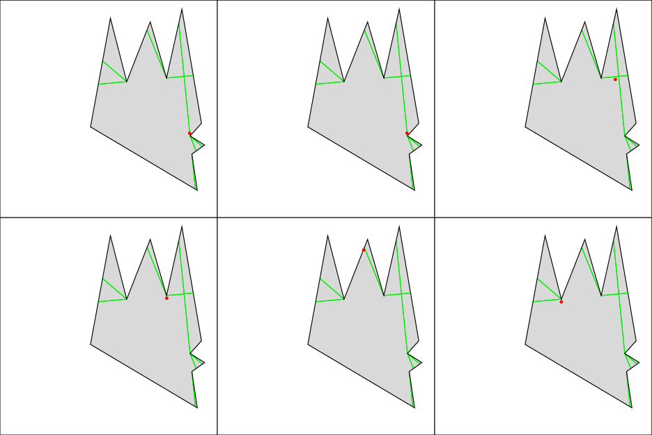Example 2: a little harder problem
Example 3: three corners to clear
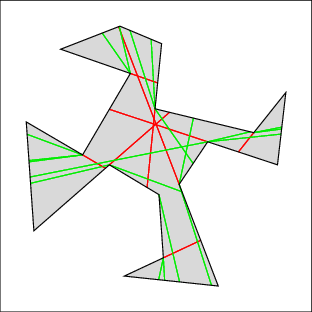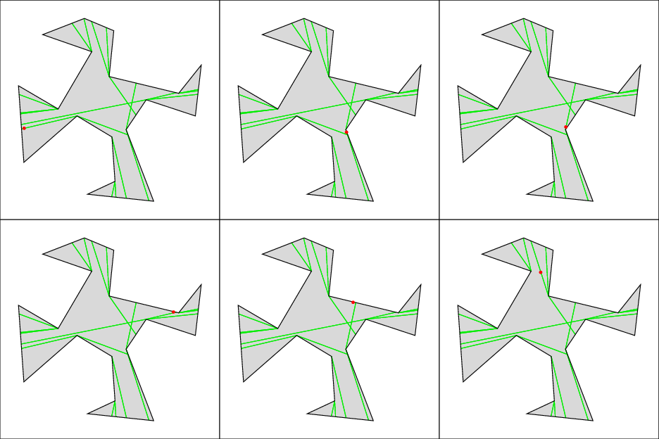Example 4: four corners to clear
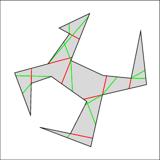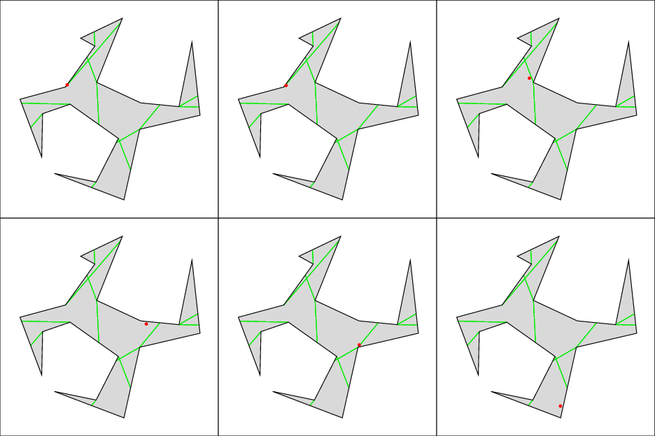Example 5: similar difficulty
Example 6: still not too hard
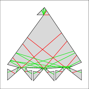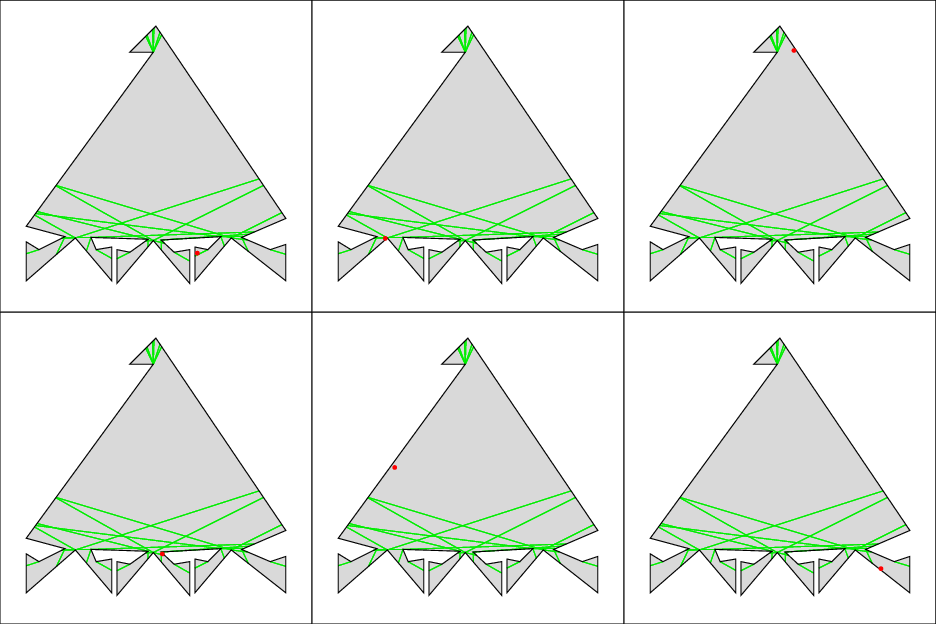Example 7: this is a tough one because the top keeps getting recontaminated
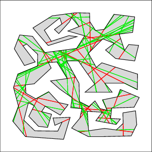Example 8: This can't be cleared by a single pursuer