Next: Computing the boundary of Up: 4.3.2 Explicitly Modeling : Previous: 4.3.2 Explicitly Modeling :
A simple algorithm for computing
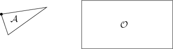
![]() exists in the case of a 2D
world that contains a convex polygonal obstacle
exists in the case of a 2D
world that contains a convex polygonal obstacle ![]() and a convex
polygonal robot
and a convex
polygonal robot ![]() [657]. This is often called the star algorithm. For this problem,
[657]. This is often called the star algorithm. For this problem,
![]() is also a convex polygon.
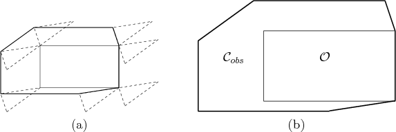
Recall that nonconvex obstacles and robots can be modeled as the union
of convex parts. The concepts discussed below can also be applied in
the nonconvex case by considering
is also a convex polygon.
Recall that nonconvex obstacles and robots can be modeled as the union
of convex parts. The concepts discussed below can also be applied in
the nonconvex case by considering
![]() as the union of convex
components, each of which corresponds to a convex component of
as the union of convex
components, each of which corresponds to a convex component of ![]() colliding with a convex component of
colliding with a convex component of ![]() .
.
The method is based on sorting normals to the edges of the polygons on
the basis of angles. The key observation is that every edge of
![]() is a translated edge from either
is a translated edge from either ![]() or
or ![]() . In fact, every
edge from
. In fact, every
edge from ![]() and
and ![]() is used exactly once in the construction of
is used exactly once in the construction of
![]() . The only problem is to determine the ordering of these edges
of
. The only problem is to determine the ordering of these edges
of
![]() . Let
. Let ![]() ,
, ![]() ,
, ![]() ,
, ![]() denote
the angles of the inward edge normals in counterclockwise order around
denote
the angles of the inward edge normals in counterclockwise order around
![]() . Let
. Let ![]() ,
, ![]() ,
, ![]() ,
, ![]() denote the
outward edge normals to
denote the
outward edge normals to ![]() . After sorting both sets of angles in
circular order around
. After sorting both sets of angles in
circular order around
![]() ,
,
![]() can be constructed incrementally
by using the edges that correspond to the sorted normals, in the order
in which they are encountered.
can be constructed incrementally
by using the edges that correspond to the sorted normals, in the order
in which they are encountered.
 |
 |
The running time of the algorithm is ![]() , in which
, in which ![]() is the
number of edges defining
is the
number of edges defining ![]() , and
, and ![]() is the number of edges defining
is the number of edges defining
![]() . Note that the angles can be sorted in linear time because they
already appear in counterclockwise order around
. Note that the angles can be sorted in linear time because they
already appear in counterclockwise order around ![]() and
and ![]() ; they
only need to be merged. If two edges are collinear, then they can be
placed end-to-end as a single edge of
; they
only need to be merged. If two edges are collinear, then they can be
placed end-to-end as a single edge of
![]() .
.