
Next: 8.5.2 Dynamic Programming with Up: 8.5.1.3 A sampling-based approach Previous: Defining new neighborhoods
The sampling-based planning algorithms in Chapter 5
were designed to terminate upon finding a solution path. In the
current setting, termination is complicated by the fact that we are
interested in solutions from all initial configurations. Since
![]() is dense, the volume of uncovered points in
is dense, the volume of uncovered points in
![]() tends
to zero. After some finite number of iterations, it would be nice to
measure the quality of the approximation and then terminate when the
desired quality is achieved. This was also possible with the
visibility sampling-based roadmap in Section 5.6.2.
Using random samples, an estimate of the fraction of
tends
to zero. After some finite number of iterations, it would be nice to
measure the quality of the approximation and then terminate when the
desired quality is achieved. This was also possible with the
visibility sampling-based roadmap in Section 5.6.2.
Using random samples, an estimate of the fraction of
![]() can be
obtained by recording the percentage of failures in obtaining a sample
in
can be
obtained by recording the percentage of failures in obtaining a sample
in
![]() that is outside of the cover. For example, if a new
neighborhood is created only once in
that is outside of the cover. For example, if a new
neighborhood is created only once in ![]() iterations, then it can be
estimated that
iterations, then it can be
estimated that ![]() percent of
percent of
![]() is covered.
High-probability bounds can also be determined. Termination
conditions are given in [983] that ensure with probability
greater than
is covered.
High-probability bounds can also be determined. Termination
conditions are given in [983] that ensure with probability
greater than ![]() that at least a fraction
that at least a fraction
![]() of
of
![]() has been covered. The constants
has been covered. The constants ![]() and
and ![]() are given
as parameters to the algorithm, and it will terminate when the
condition has been satisfied using rigorous statistical tests. If
deterministic sampling is used, then termination can be made to occur
based on the dispersion, which indicates the largest ball in
are given
as parameters to the algorithm, and it will terminate when the
condition has been satisfied using rigorous statistical tests. If
deterministic sampling is used, then termination can be made to occur
based on the dispersion, which indicates the largest ball in
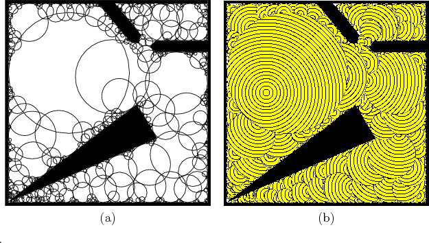
![]() that does not contain the center of another neighborhood. One problem
with volume-based criteria, such as those suggested here, is that
there is no way to ensure that the cover preserves the connectivity of
that does not contain the center of another neighborhood. One problem
with volume-based criteria, such as those suggested here, is that
there is no way to ensure that the cover preserves the connectivity of
![]() . If two portions of
. If two portions of
![]() are connected by a narrow
passage, the cover may miss a neighborhood that has very small volume
yet is needed to connect the two portions.
are connected by a narrow
passage, the cover may miss a neighborhood that has very small volume
yet is needed to connect the two portions.
 |
Steven M LaValle 2012-04-20