Next: 9.3 Two-Player Zero-Sum Games Up: 9.2.4 Examples of Optimal Previous: A Bayesian classifier
Another important application of the decision-making framework of this
section is parameter estimation [89,268]. In this
case, nature selects a parameter,
![]() , and
, and
![]() represents a parameter space. Through one or more
independent trials, some observations are obtained. Each observation
should ideally be a direct measurement of
represents a parameter space. Through one or more
independent trials, some observations are obtained. Each observation
should ideally be a direct measurement of ![]() , but imperfections
in the measurement process distort the observation. Usually,
, but imperfections
in the measurement process distort the observation. Usually,
![]() , and in many cases,
, and in many cases,
![]() . The robot action is to
guess the parameter that was chosen by nature. Hence,
. The robot action is to
guess the parameter that was chosen by nature. Hence,
![]() .
In most applications, all of the spaces are continuous subsets of
.
In most applications, all of the spaces are continuous subsets of
![]() . The cost function is designed to increase as the error,
. The cost function is designed to increase as the error,
![]() , becomes larger.
, becomes larger.
| (9.35) |
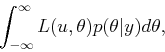
Suppose that a Bayesian approach is taken. The prior probability
density ![]() is given as uniform over an interval
is given as uniform over an interval
![]() . An observation is received, but it is noisy. The noise
can be modeled as a second action of nature, as described in Section
9.2.3. This leads to a density
. An observation is received, but it is noisy. The noise
can be modeled as a second action of nature, as described in Section
9.2.3. This leads to a density
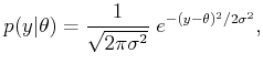
![]() . Suppose
that the noise is modeled with a Gaussian, which results in
. Suppose
that the noise is modeled with a Gaussian, which results in
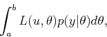
The optimal parameter estimate based on ![]() is obtained by selecting
is obtained by selecting
![]() to minimize
to minimize
 |
(9.37) |
 |
(9.38) |
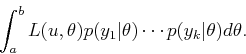
If a sequence, ![]() ,
, ![]() ,
, ![]() , of independent observations is
obtained, then (9.39) is replaced by
, of independent observations is
obtained, then (9.39) is replaced by
Steven M LaValle 2012-04-20