9.4.2 More Than Two Players

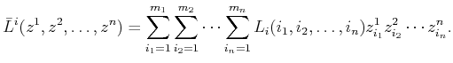
The ideas of Section 9.4.1 easily generalize to any number of players. The main difficulty is that complicated notation makes the concepts appear more difficult. Keep in mind, however, that there are no fundamental differences. A nonzero-sum game with $n$ players is formulated as follows.

Formulation 9..9 (An $n$-Player Nonzero-Sum Game)  

1. A set of $n$ players, ${{\rm P}_1}$, ${{\rm P}_2}$, $\ldots$, ${{\rm P}_n}$.
2. For each player ${{\rm P}_i}$, a finite, nonempty set $U^i$ called the action space for ${{\rm P}_i}$. For convenience, assume that each $U^i$ is a set of consecutive integers from $1$ to $\vert U^i\vert$. Each $u^i \in U^i$ is referred to as an action of ${{\rm P}_i}$.
3. For each player ${{\rm P}_i}$, a function, $L_i: U^1 \times U^2 \times \cdots \times U^n \rightarrow {\mathbb{R}}\cup \{\infty\}$ called the cost function for ${{\rm P}_i}$.

A matrix formulation of the costs is no longer possible because there are too many dimensions. For example, if $n=3$ and $\vert U^i\vert = 2$ for each player, then $L_i(u^1,u^2,u^3)$ is specified by a $2 \times 2 \times 2$ cube of $8$ entries. Three of these cubes are needed to specify the game. Thus, it may be helpful to just think of $L_i$ as a multivariate function and avoid using matrices.^9.4

The Nash equilibrium idea generalizes by requiring that each ${{\rm P}_i}$ experiences no regret, given the actions chosen by the other $n-1$ players. Formally, a set $(u^{1*},\ldots,u^{n*})$ of actions is said to be a (deterministic) Nash equilibrium if

$$L_i(u^{1*},\ldots,u^{i*},\ldots,u^{n*}) = \min_{u^i \in U^i} \Big\{ L_i(u^{1*},\ldots,u^{(i-1)*},u^{i},u^{(i+1)*},\ldots,u^{n*}) \Big\}$$ (9.79)

for every $i \in \{1,\ldots,n\}$.

For $n > 2$, any of the situations summarized at the end of Section 9.4.1 can occur. There may be no deterministic Nash equilibria or multiple Nash equilibria. The definition of an admissible Nash equilibrium is extended by defining the notion of better over $n$-dimensional cost vectors. Once again, the minimal vectors with respect to the resulting partial ordering are considered admissible (or Pareto optimal). Unfortunately, multiple admissible Nash equilibria may still exist.

It turns out that for any game under Formulation 9.9, there exists a randomized Nash equilibrium. Let $z^i$ denote a randomized strategy for ${{\rm P}_i}$. The expected cost for each ${{\rm P}_i}$ can be expressed as

$${\bar{L}}^i(z^1,z^2,\ldots,z^n) = \sum_{i_1 = 1}^{m_1} \sum_{i_2 ... ..._{i_n = 1}^{m_n} L_i(i_1,i_2,\ldots,i_n) z^1_{i_1} z^2_{i_2} \cdots z^n_{i_n} .$$ (9.80)

Let $Z^i$ denote the space of randomized strategies for ${{\rm P}_i}$. An assignment, $(z^{1*},\ldots,z^{n*})$, of randomized strategies to all of the players is called a randomized Nash equilibrium if

$${\bar{L}}^i(z^{1*},\ldots,z^{i*},\ldots,z^{n*}) = \min_{z^i \in Z... ...g\{ {\bar{L}}^i(z^{1*},\ldots,z^{(i-1)*},z^{i},z^{(i+1)*},\ldots,z^{n*}) \Big\}$$ (9.81)

for all $i \in \{1,\ldots,n\}$.

As might be expected, computing a randomized Nash equilibrium for $n > 2$ is even more challenging than for $n=2$. The method of Example 9.20 can be generalized to $n$-player games; however, the expressions become even more complicated. There are $n$ equations, each of which appears linear if the randomized strategies are fixed for the other $n-1$ players. The result is a collection of $n$-degree polynomials over which $n$ optimization problems must be solved simultaneously.

Example 9..21 (A Three-Player Nonzero-Sum Game)   Suppose there are three players, ${{\rm P}_1}$, ${{\rm P}_2}$, and ${{\rm P}_3}$, each of which has two actions, $1$ and $2$. A deterministic strategy is specified by a vector such as $(1,2,1)$, which indicates $u^1 = 1$, $u^2 = 2$, and $u^3 = 1$.

Now some costs will be defined. For convenience, let

$$L(i,j,k) = \Big( L_1(i,j,k),\;L_2(i,j,k),\;L_3(i,j,k)\Big)$$ (9.82)

for each $i,j,k \in \{1,2\}$. Let the costs be

$$L(1,1,1) = (1,1,-2) \qquad L(1,1,2) = (-4,3,1)$$

$$L(1,2,1) = (2,-4,2) \qquad L(1,2,2) = (-5,-5,10)$$ (9.83)

$$L(2,1,1) = (3,-2,-1) \qquad L(2,1,2) = (-6,-6,12)$$

$$L(2,2,1) = (2,2,-4) \qquad L(2,2,2) = (-2,3,-1) .$$

There are two deterministic Nash equilibria, which yield the costs $(2,-4,2)$ and $(3,-2,-1)$. These can be verified using (9.79). Each player is satisfied with the outcome given the actions chosen by the other players. Unfortunately, both Nash equilibria are both admissible. Therefore, some collaboration would be needed between the players to ensure that no regret will occur. $\blacksquare$