Next: Using the plan Up: 10.2.1 Value Iteration Previous: Probabilistic case
If the maximum number of stages is fixed in the problem definition,
then convergence is assured. Suppose, however, that there is no limit
on the number of stages. Recall from Section 2.3.2 that
each value iteration increases the total path length by one. The
actual stage indices were not important in backward dynamic
programming because arbitrary shifting of indices does not affect the
values. Eventually, the algorithm terminated because optimal
cost-to-go values had been computed for all reachable states from the
goal. This resulted in a stationary cost-to-go function because
the values no longer changed. States that are reachable from the goal
converged to finite values, and the rest remained at infinity. The
only problem that prevents the existence of a stationary cost-to-go
function, as mentioned in Section 2.3.2, is negative cycles
in the graph. In this case, the best plan would be to loop around the
cycle forever, which would reduce the cost to ![]() .
.
In the current setting, a stationary cost-to-go function once again
arises, but cycles once again cause difficulty in convergence. The
situation is, however, more complicated due to the influence of
nature. It is helpful to consider a plan-based state transition
graph,
![]() . First consider the nondeterministic case. If
there exists a plan
. First consider the nondeterministic case. If
there exists a plan ![]() from some state
from some state ![]() for which all
possible actions of nature cause the traversal of cycles that
accumulate negative cost, then the optimal cost-to-go at
for which all
possible actions of nature cause the traversal of cycles that
accumulate negative cost, then the optimal cost-to-go at ![]() converges to
converges to ![]() , which prevents the value iterations from
terminating. These cases can be detected in advance, and each such
initial state can be avoided (some may even be in a different
connected component of the state space).
, which prevents the value iterations from
terminating. These cases can be detected in advance, and each such
initial state can be avoided (some may even be in a different
connected component of the state space).
 |
It is also possible that there are unavoidable positive cycles. In
Section 2.3.2, the cost-to-go function behaved differently
depending on whether the goal set was reachable. Due to nature, the
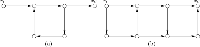
goal set may be possibly reachable or guaranteed reachable, as
illustrated in Figure 10.2. To be possibly reachable
from some initial state, there must exist a plan, ![]() , for which
there exists a sequence of nature actions that will lead the state
into the goal set. To be guaranteed reachable, the goal must be
reached in spite of all possible sequences of nature actions.
If the goal is possibly reachable, but not guaranteed reachable, from
some state
, for which
there exists a sequence of nature actions that will lead the state
into the goal set. To be guaranteed reachable, the goal must be
reached in spite of all possible sequences of nature actions.
If the goal is possibly reachable, but not guaranteed reachable, from
some state ![]() and all edges have positive cost, then the
cost-to-go value of
and all edges have positive cost, then the
cost-to-go value of ![]() tends to infinity as the value iterations
are repeated. For example, every plan-based state transition graph
may contain a cycle of positive cost, and in the worst case, nature
may cause the state to cycle indefinitely. If convergence of the
value iterations is only evaluated at states from which the goal set
is guaranteed to be reachable, and if there are no negative cycles,
then the algorithm should terminate when all cost-to-go values remain
unchanged.
tends to infinity as the value iterations
are repeated. For example, every plan-based state transition graph
may contain a cycle of positive cost, and in the worst case, nature
may cause the state to cycle indefinitely. If convergence of the
value iterations is only evaluated at states from which the goal set
is guaranteed to be reachable, and if there are no negative cycles,
then the algorithm should terminate when all cost-to-go values remain
unchanged.
For the probabilistic case, there are three situations:
The third situation is unique to the probabilistic setting. This is
caused by positive or negative cycles in
![]() for which the
edges have probabilities in
for which the
edges have probabilities in ![]() . The optimal plan may even have
such cycles. As the value iterations consider longer and longer
paths, a cycle may be traversed more times. However, each time the
cycle is traversed, the probability diminishes. The probabilities
diminish exponentially in terms of the number of stages, whereas the
costs only accumulate linearly. The changes in the cost-to-go
function gradually decrease and converge only to stationary values as
the number of iterations tends to infinity. If some approximation
error is acceptable, then the iterations can be terminated once the
maximum change over all of
. The optimal plan may even have
such cycles. As the value iterations consider longer and longer
paths, a cycle may be traversed more times. However, each time the
cycle is traversed, the probability diminishes. The probabilities
diminish exponentially in terms of the number of stages, whereas the
costs only accumulate linearly. The changes in the cost-to-go
function gradually decrease and converge only to stationary values as
the number of iterations tends to infinity. If some approximation
error is acceptable, then the iterations can be terminated once the
maximum change over all of ![]() is within some
is within some ![]() threshold.
The required number of value iterations to obtain a solution of the
desired quality depends on the probabilities of following the cycles
and on their costs. If the probabilities are lower, then the
algorithm converges sooner.
threshold.
The required number of value iterations to obtain a solution of the
desired quality depends on the probabilities of following the cycles
and on their costs. If the probabilities are lower, then the
algorithm converges sooner.
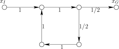 |
The expected cost from ![]() is straightforward to compute. With
probability
is straightforward to compute. With
probability ![]() , the cost to reach
, the cost to reach ![]() is
is ![]() . With
probability
. With
probability ![]() , the cost is
, the cost is ![]() . With probability
. With probability ![]() , the cost
is
, the cost
is ![]() . Each time another cycle is taken, the cost increases by
. Each time another cycle is taken, the cost increases by ![]() ,
but the probability is cut in half. This leads to the infinite series
,
but the probability is cut in half. This leads to the infinite series
Even though the cost converges to a finite value, this only occurs in
the limit. An infinite number of value iterations would theoretically
be required to obtain this result. For most applications, an
approximate solution suffices, and very high precision can be obtained
with a small number of iterations (e.g., after ![]() iterations, the
change is on the order of one-billionth). Thus, in general, it is
sensible to terminate the value iterations after the maximum
cost-to-go change is less than a threshold based directly on
precision.
iterations, the
change is on the order of one-billionth). Thus, in general, it is
sensible to terminate the value iterations after the maximum
cost-to-go change is less than a threshold based directly on
precision.
Note that if nondeterministic uncertainty is used, then the value
iterations do not converge because, in the worst case, nature will
cause the state to cycle forever. Even though the goal is not
guaranteed reachable, the probabilistic uncertainty model allows
reasonable solutions.
![]()
Steven M LaValle 2012-04-20