Next: 10.5.1.3 Converting the tree Up: 10.5.1 Game Trees Previous: 10.5.1.1 Determining a security
The security plan for
![]() constitutes a valid solution to the game
under the alternating play model.
constitutes a valid solution to the game
under the alternating play model.
![]() has only to choose an optimal
response to the plan of
has only to choose an optimal
response to the plan of
![]() at each stage. Under the stage-by-stage
model, the ``solution'' concept is a saddle point, which occurs when
the upper and lower values coincide. The procedure just described
could be used to determine the value and corresponding plans; however,
what happens when the values do not coincide? In this case, randomized security plans should be
developed for the players. As in the case of a single-stage game, a
randomized upper value
at each stage. Under the stage-by-stage
model, the ``solution'' concept is a saddle point, which occurs when
the upper and lower values coincide. The procedure just described
could be used to determine the value and corresponding plans; however,
what happens when the values do not coincide? In this case, randomized security plans should be
developed for the players. As in the case of a single-stage game, a
randomized upper value
![]() and a randomized lower
value
and a randomized lower
value
![]() are obtained. In the space of randomized plans, it
turns out that a saddle point always exists. This implies that the
game always has a randomized value,
are obtained. In the space of randomized plans, it
turns out that a saddle point always exists. This implies that the
game always has a randomized value,
![]() . This saddle point can be computed from the bottom up, in a
manner similar to the method just used to compute security plans.
. This saddle point can be computed from the bottom up, in a
manner similar to the method just used to compute security plans.
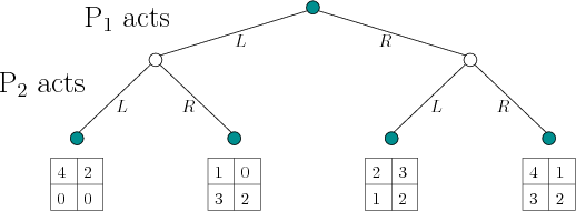
Return to the example in Figure 10.13. This game actually
has a deterministic saddle point, as indicated previously. It still,
however, serves as a useful illustration of the method because any
deterministic plan can once again be interpreted as a special case of
a randomized plan (all of the probability mass is placed on a single
action). Consider the bottom four subtrees of Figure 10.13,
which are obtained by using only the last two levels of decision
vertices. In each case,
![]() and
and
![]() must act in parallel to end the
sequential game. Each subtree can be considered as a matrix game
because the costs are immediately obtained after the two players act.
must act in parallel to end the
sequential game. Each subtree can be considered as a matrix game
because the costs are immediately obtained after the two players act.
 |
 |
Steven M LaValle 2012-04-20