Next: 10.5.3 Other Sequential Games Up: 10.5.2 Sequential Games on Previous: Saddle points in a
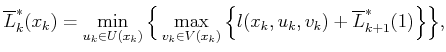
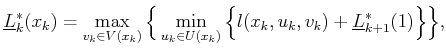
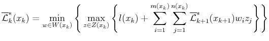
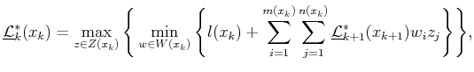
A value-iteration method can be derived by adapting the derivation that was applied to (10.33) to instead apply to (10.108). This leads to the dynamic programming recurrence
Starting from the final stage, ![]() , the upper and lower values are
determined directly from the cost function:
, the upper and lower values are
determined directly from the cost function:
Suppose for now that
![]() for all
for all ![]() . The value iterations proceed in the usual way from
. The value iterations proceed in the usual way from ![]() down to
down to ![]() . Again, suppose that at every stage,
. Again, suppose that at every stage,
![]() for all
for all ![]() . Note that
. Note that ![]() can
be written in the place of
can
be written in the place of
![]() and
and
![]() in
(10.110) and (10.111) because it is assumed
that the upper and lower values coincide. If they do not, then the
method fails because randomized plans are needed to obtain a
randomized saddle point.
in
(10.110) and (10.111) because it is assumed
that the upper and lower values coincide. If they do not, then the
method fails because randomized plans are needed to obtain a
randomized saddle point.
Once the resulting values are computed from each
![]() , a
security plan
, a
security plan ![]() for
for
![]() is defined for each
is defined for each
![]() and
and ![]() as any action
as any action ![]() that satisfies the
that satisfies the ![]() in (10.110). A security plan
in (10.110). A security plan ![]() is similarly
defined for
is similarly
defined for
![]() by applying any action
by applying any action ![]() that satisfies the
that satisfies the
![]() in (10.111).
in (10.111).
Now suppose that there exists no deterministic saddle point from one
or more initial states. To avoid regret, randomized security plans
must be developed. These follow by direct extension of the randomized
security strategies from Section 9.3.3. The vectors
![]() and
and ![]() will be used here to denote probability distributions over
will be used here to denote probability distributions over
![]() and
and ![]() , respectively. The probability vectors are selected
from
, respectively. The probability vectors are selected
from ![]() and
and ![]() , which correspond to the set of all probability
distributions over
, which correspond to the set of all probability
distributions over ![]() and
and ![]() , respectively. For notational
convenience, assume
, respectively. For notational
convenience, assume
![]() and
and
![]() , in which
, in which ![]() and
and ![]() are positive integers.
are positive integers.
Recall (9.61) and (9.62), which defined the
randomized upper and lower values of a single-stage game. This idea
is generalized here to randomized upper and lower value of a sequential game. Their definitions are similar to (10.108)
and (10.109), except that: 1) the alternating ![]() 's and
's and
![]() 's are taken over probability distributions on the space of
actions, and 2) the expected cost is used.
's are taken over probability distributions on the space of
actions, and 2) the expected cost is used.
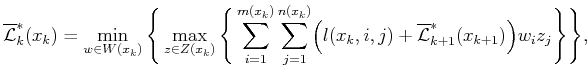
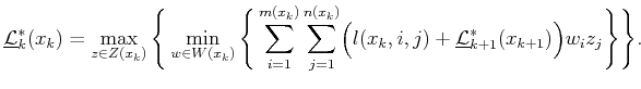
The dynamic programming principle can be applied to the randomized upper value to derive
In many games, the cost term may depend only on the state:
![]() for all
for all ![]() ,
,
![]() and
and
![]() . In this case,
(10.113) and (10.114) simplify to
. In this case,
(10.113) and (10.114) simplify to
Value iteration can be performed over the equations above to obtain
the randomized values of the sequential game. Since the upper and
lower values are always the same, there is no need to check for
discrepancies between the two. In practice, it is best in every
evaluation of (10.113) and (10.114) (or their
simpler forms) to first check whether a deterministic saddle exists
from ![]() . Whenever one does not exist, the linear programming
problem formulated in Section 9.3.3 must be solved to
determine the value and the best randomized plan for each player.
This can be avoided if a deterministic saddle exists from the current
state and stage.
. Whenever one does not exist, the linear programming
problem formulated in Section 9.3.3 must be solved to
determine the value and the best randomized plan for each player.
This can be avoided if a deterministic saddle exists from the current
state and stage.
Steven M LaValle 2012-04-20