10.6.2 Motion planning with nature

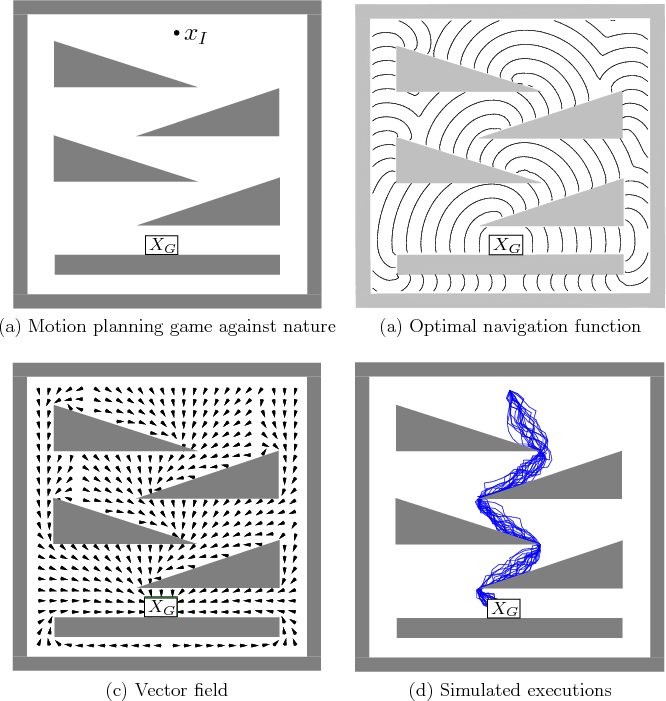
Figure 10.20: (a) A 2D planning problem is shown in which nature is probabilistic (uniform density over an interval of angles) and can interfere with the direction of motion. Contact with obstacles is actually allowed in this problem. (b) Level sets of the computed, optimal cost-to-go (navigation) function. (c) The vector field derived from the navigation function. (d) Several dozen execution trials are superimposed [605].

Recall from Section 8.5.2 that value iteration with interpolation can be applied to motion planning problems that are approximated in discrete time. Nature can even be introduced into the discrete-time approximation. For example, (8.62) can be replaced by

$$x(t + \Delta t) = x(t) + \Delta t \; (u + \theta),$$ (10.123)

in which $\theta$ is chosen from a bounded set, $\Theta(x,u)$. Using (10.124), value iterations can be performed as described so far. An example of a 2D motion planning problem under this model using probabilistic uncertainty is shown in Figure 10.20. It is interesting that when the plan is executed from a fixed initial state, a different trajectory is obtained each time. The average cost over multiple executions, however, is close to the expected optimum.

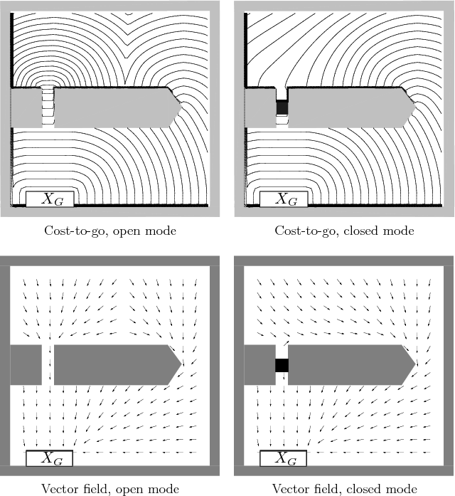
Figure 10.21: Level sets of the optimal navigation function and resulting vector field are shown for a stochastic, hybrid motion planning problem. There are two modes, which correspond to whether a door is closed. The goal is to reach the rectangle at the bottom left [613]

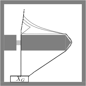
Figure 10.22: Several executions from the same initial state are shown. A different trajectory results each time because of the different times when the door is open or closed.

Interesting hybrid system examples can be made in which nature is only allowed to interfere with the mode. Recall Formulation 7.3 from Section 7.3. Nature can be added to yield the following formulation.

Formulation 10..5 (Hybrid System Motion Planning with Nature)  

1. Assume all of the definitions from Formulation 7.3, except for the transition functions, $f_m$ and $f$. The state is represented as $x = (q,m)$.
2. A finite nature action space $\Theta(x,u)$ for each $x \in X$ and $u \in U(x)$.
3. A mode transition function $f_m$ that produces a mode $f_m(x,u,\theta)$ for every $x \in X$, $u \in U(x)$, and $\theta \in \Theta(x,u)$.
4. A state transition function $f$ that is derived from $f_m$ by changing the mode and holding the configuration fixed. Thus, $f((q,m),u,\theta) = (q,f_m(q,m,\theta))$ (the only difference with respect to Formulation 7.3 is that $\theta$ has been included).
5. An unbounded time interval $T = [0,\infty)$.
6. A continuous-time cost-functional,

   $$L({\tilde{x}}_{t_F},{\tilde{u}}_{t_F}) = \int_0^{t_F} l(x(t),u(t)) dt + l_F(x(t_F)).$$ (10.124)

   
   

Value iteration proceeds in the same way for such hybrid problems. Interpolation only needs to be performed over the configuration space. Along the mode ``axis'' no interpolation is needed because the mode set is already finite. The resulting computation time grows linearly in the number of modes. A 2D motion planning example for a point robot, taken from [613], is shown in Figures 10.21 and 10.22. In this case, the environment contains a door that is modeled as a stationary Markov process. The configuration space is sampled using a $40 \times 40$ grid. There are two modes: door open or door closed. Thus, the configuration space has two layers, one for each mode. The robot wishes to minimize the expected time to reach the goal. The navigation function for each layer cannot be computed independently because each takes into account the transition probabilities for the mode. For example, if the door is almost always open, then its plan would be different from one in which the door is almost always closed. If the door is almost always open, then the robot should go toward the door, even if it is currently closed, because it is highly likely that it will open soon. Numerous variations can be made on this example. More modes could be added, and other interpretations are possible, such as hazardous regions and shelters (the mode might be imagined as rain occurring and the robot must run for shelter) or requests to deliver objects [613,870,871].