Next: 11.2.4 Limited-Memory Information Spaces Up: 11.2 Derived Information Spaces Previous: 11.2.2 Nondeterministic Information Spaces
This section defines the I-map
![]() from Figure
11.3, which converts each history I-state into a
probability distribution over
from Figure
11.3, which converts each history I-state into a
probability distribution over ![]() . A Markov, probabilistic model is
assumed in the sense that the actions of nature only depend on the
current state and action, as opposed to state or action histories. The
set union and intersection of (11.30) and
(11.31) are replaced in this section by marginalization
and Bayes' rule, respectively. In a sense, these are the probabilistic
equivalents of union and intersection. It will be very helpful to
compare the expressions from this section to those of Section
11.2.2.
. A Markov, probabilistic model is
assumed in the sense that the actions of nature only depend on the
current state and action, as opposed to state or action histories. The
set union and intersection of (11.30) and
(11.31) are replaced in this section by marginalization
and Bayes' rule, respectively. In a sense, these are the probabilistic
equivalents of union and intersection. It will be very helpful to
compare the expressions from this section to those of Section
11.2.2.
Rather than write
![]() , standard probability notation
will be applied to obtain
, standard probability notation
will be applied to obtain
![]() . Most expressions in this
section of the form
. Most expressions in this
section of the form
![]() have an analogous expression in
Section 11.2.2 of the form
have an analogous expression in
Section 11.2.2 of the form
![]() . It is helpful to
recognize the similarities.
. It is helpful to
recognize the similarities.
The first step is to construct probabilistic versions of ![]() and
and ![]() .
These are
.
These are
![]() and
and
![]() , respectively. The
latter term was given in Section 10.1.1. To obtain
, respectively. The
latter term was given in Section 10.1.1. To obtain
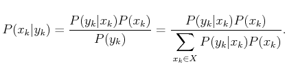
![]() , recall from Section 11.1.1 that
, recall from Section 11.1.1 that
![]() is easily derived from
is easily derived from
![]() . To obtain
. To obtain
![]() ,
Bayes' rule is applied:
,
Bayes' rule is applied:
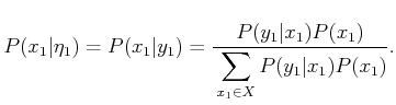
Now consider defining probabilistic I-states. Each is a probability
distribution over ![]() and is written as
and is written as
![]() . The initial
condition produces
. The initial
condition produces ![]() . As for the nondeterministic case,
probabilistic I-states can be computed inductively. For the base
case, the only new piece of information is
. As for the nondeterministic case,
probabilistic I-states can be computed inductively. For the base
case, the only new piece of information is ![]() . Thus, the
probabilistic I-state,
. Thus, the
probabilistic I-state,
![]() , is
, is
![]() . This is
computed by letting
. This is
computed by letting ![]() in (11.35) to yield
in (11.35) to yield
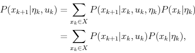
Now consider the inductive step by assuming that
![]() is
given. The task is to determine
is
given. The task is to determine
![]() , which is
equivalent to
, which is
equivalent to
![]() . As in Section
11.2.2, this will proceed in two parts by first considering
the effect of
. As in Section
11.2.2, this will proceed in two parts by first considering
the effect of ![]() , followed by
, followed by ![]() . The first step is to
determine
. The first step is to
determine
![]() from
from
![]() . First, note
that
. First, note
that
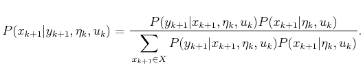
The next step is to take into account the observation ![]() .
This is accomplished by making a version of (11.35) that is
conditioned on the information accumulated so far:
.
This is accomplished by making a version of (11.35) that is
conditioned on the information accumulated so far: ![]() and
and ![]() .
Also,
.
Also, ![]() is replaced with
is replaced with ![]() . The result is
. The result is
The probabilistic I-space
![]() (shown in Figure
11.3) is the set of all probability distributions over
(shown in Figure
11.3) is the set of all probability distributions over
![]() . The update expressions, (11.38) and
(11.39), establish that the I-map
. The update expressions, (11.38) and
(11.39), establish that the I-map
![]() is
sufficient, which means that the planning problem can be expressed
entirely in terms of
is
sufficient, which means that the planning problem can be expressed
entirely in terms of
![]() , instead of maintaining histories. A
goal region can be specified as constraints on the probabilities. For
example, from some particular
, instead of maintaining histories. A
goal region can be specified as constraints on the probabilities. For
example, from some particular ![]() , the goal might be to reach
any probabilistic I-state for which
, the goal might be to reach
any probabilistic I-state for which
![]() .
.
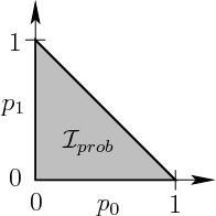 |
The triangular region in
![]() is an uncountably infinite set, even
though the history I-space is countably infinite for a fixed initial
condition. This may seem strange, but there is no mistake because for
a fixed initial condition, it is generally impossible to reach all of
the points in
is an uncountably infinite set, even
though the history I-space is countably infinite for a fixed initial
condition. This may seem strange, but there is no mistake because for
a fixed initial condition, it is generally impossible to reach all of
the points in
![]() . If the initial condition can be any point
in
. If the initial condition can be any point
in
![]() , then all of the probabilistic I-space is covered
because
, then all of the probabilistic I-space is covered
because
![]() , in which
, in which
![]() is the initial condition
space..
is the initial condition
space..
![]()
Steven M LaValle 2012-04-20