Next: 10.4.2 Evaluating a Plan Up: 10.4.1 The General Philosophy Previous: Terminology
The framework is usually applied to infinite-horizon problems under
probabilistic uncertainty. The discounted-cost model is most popular;
however, we will mostly work with Formulation 10.1 because
it is closer to the main theme of this book. It has been assumed so
far that when planning under Formulation 10.1, all model
components are known, including
![]() . This can be
considered as a traditional framework, in which there are three
general phases:
. This can be
considered as a traditional framework, in which there are three
general phases:
The simulation-based framework combines all three of these phases into
one. Learning, planning, and execution are all conducted by a machine
that initially knows nothing about the state transitions or even the
cost terms. Ideally, the machine should be connected to a physical
environment for which the Markov model holds. However, in nearly all
implementations, the machine is instead connected to a Monte Carlo
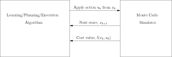
simulator as shown in Figure 10.11. Based on the current
state, the algorithm sends an action, ![]() , to the simulator, and the
simulator computes its effect by sampling according to its internal
probability distributions. Obviously, the designer of the simulator
knows the transition probabilities, but these are not given directly
to the planning algorithm. The simulator then sends the next state,
, to the simulator, and the
simulator computes its effect by sampling according to its internal
probability distributions. Obviously, the designer of the simulator
knows the transition probabilities, but these are not given directly
to the planning algorithm. The simulator then sends the next state,
![]() , and cost,
, and cost,
![]() , back to the algorithm.
, back to the algorithm.
 |
For simplicity,
![]() is used instead of allowing the cost to
depend on the particular nature action, which would yield
is used instead of allowing the cost to
depend on the particular nature action, which would yield
![]() . The explicit characterization of nature is
usually not needed in this framework. The probabilities
. The explicit characterization of nature is
usually not needed in this framework. The probabilities
![]() are directly learned without specifying nature
actions. It is common to generalize the cost term from
are directly learned without specifying nature
actions. It is common to generalize the cost term from
![]() to
to
![]() , but this is avoided here for notational
convenience. The basic ideas remain the same, and only slight
variations of the coming equations are needed to handle this
generalization.
, but this is avoided here for notational
convenience. The basic ideas remain the same, and only slight
variations of the coming equations are needed to handle this
generalization.
The simulator is intended to simulate ``reality,'' in which the machine interacts with the physical world. It replaces the environment in Figure 1.16b from Section 1.4. Using the interpretation of that section, the algorithms presented in this context can be considered as a plan as shown in Figure 1.18b. If the learning component is terminated, then the resulting feedback plan can be programmed into another machine, as shown in Figure 1.18a. This step is usually not performed, however, because often it is assumed that the machine continues to learn over its lifetime.
One of the main issues is exploration vs. exploitation [930]. Some repetitive exploration of the state space is needed to gather enough data that reliably estimate the model. For true theoretical convergence, each state-action pair must be tried infinitely often. On the other hand, information regarding the model should be exploited to efficiently accomplish tasks. These two goals are often in conflict. Focusing too much on exploration will not optimize costs. Focusing too much on exploitation may prevent useful solutions from being developed because better alternatives have not yet been discovered.
Steven M LaValle 2012-04-20