Next: 10.4.3 Q-Learning: Computing an Up: 10.4.2 Evaluating a Plan Previous: 10.4.2 Evaluating a Plan
Rather than waiting until the end of each trial to compute ![]() ,
it is possible to update each state,
,
it is possible to update each state, ![]() , immediately after it is
visited and
, immediately after it is
visited and
![]() is received from the simulator. This leads
to a well-known method of estimating the cost-to-go called
temporal differences [929]. It is very similar to the
method already given but somewhat more complicated. It will be
introduced here because the method frequently appears in reinforcement
learning literature, and an extension of it leads to a nice
simulation-based method for updating the estimated cost-to-go.
is received from the simulator. This leads
to a well-known method of estimating the cost-to-go called
temporal differences [929]. It is very similar to the
method already given but somewhat more complicated. It will be
introduced here because the method frequently appears in reinforcement
learning literature, and an extension of it leads to a nice
simulation-based method for updating the estimated cost-to-go.
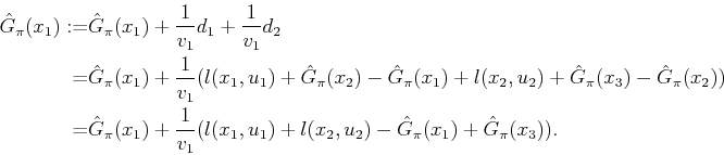
Once again, consider the sequence ![]() ,
, ![]() ,
, ![]() ,
, ![]() generated by a trial. Let
generated by a trial. Let ![]() denote a temporal
difference, which is defined as
denote a temporal
difference, which is defined as
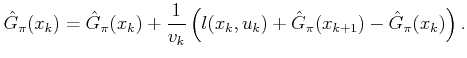
Let ![]() denote the number of times that
denote the number of times that ![]() has been visited so
far, for each
has been visited so
far, for each
![]() , including previous trials and the
current visit. The following update algorithm can be used during the
trial. When
, including previous trials and the
current visit. The following update algorithm can be used during the
trial. When ![]() is reached, the value at
is reached, the value at ![]() is updated as
is updated as
 |
(10.87) |
 |
(10.88) |
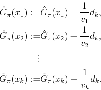
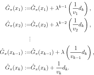
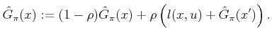
The temporal difference method presented so far can be generalized in
a way that often leads to faster convergence in practice. Let
![]() be a specified parameter. The
be a specified parameter. The
![]() temporal difference method replaces the equations in (10.91)
with
temporal difference method replaces the equations in (10.91)
with
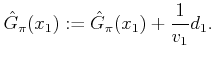
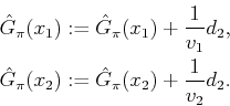
Another interesting special case is ![]() , which becomes
, which becomes
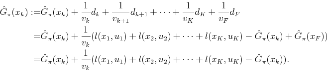
One source of intuition about why (10.94) works is that it is
a special case of a stochastic iterative algorithm or the Robbins-Monro algorithm [88,97,566]. This
is a general statistical estimation technique that is used for solving
systems of the form ![]() by using a sequence of samples. Each
sample represents a measurement of
by using a sequence of samples. Each
sample represents a measurement of ![]() using Monte Carlo
simulation. The general form of this iterative approach is to update
using Monte Carlo
simulation. The general form of this iterative approach is to update
![]() as
as
A general approach to obtaining
![]() can be derived within the
stochastic iterative framework by
generalizing
can be derived within the
stochastic iterative framework by
generalizing ![]() :
:
It may appear incorrect that the update equation does not take into account the transition probabilities. It turns out that they are taken into account in the simulation process because transitions that are more likely to occur have a stronger effect on (10.96). The same thing occurs when the mean of a nonuniform probability density function is estimated by using samples from the distribution. The values that occur with higher frequency make stronger contributions to the average, which automatically gives them the appropriate weight.