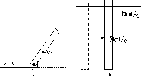
Figure 2.7 shows two different ways in which a pair of
2D links can be attached. The place at which the links are attached
is called a joint. In Figure 2.7.a, a
revolute joint is shown, in which one link is capable only of
rotation with respect to the other. In Figure 2.7.b, a
prismatic joint is shown, in which one link translates along the
other. Each type of joint removes two degrees of freedom from the
pair of bodies. For example, consider a revolute joint that connects
![]() to
to ![]() . Assume that the point (0,0) in the model for
. Assume that the point (0,0) in the model for
![]() is permanently fixed to a point (xa,ya) on
is permanently fixed to a point (xa,ya) on ![]() . This
implies that the translation of
. This
implies that the translation of ![]() will be completely determined
once xa and ya are given. Note that xa and ya are
functions of x1, y1, and
will be completely determined
once xa and ya are given. Note that xa and ya are
functions of x1, y1, and ![]() . This implies that
. This implies that ![]() and
and ![]() have a total of four degrees of freedom when attached. The
independent parameters are x1, x2,
have a total of four degrees of freedom when attached. The
independent parameters are x1, x2, ![]() , and
, and ![]() .The task in the remainder of this section is to determine exactly how
the models of
.The task in the remainder of this section is to determine exactly how
the models of ![]() ,
, ![]() ,
, ![]() ,
, ![]() are transformed, and
give the expressions in terms of these independent parameters.
are transformed, and
give the expressions in terms of these independent parameters.
 |
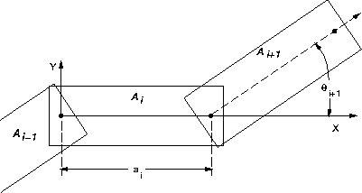
Consider the case of a kinematic chain in which each pair of links is
attached by a revolute joint. The first task is to specify the
geometric model for each link, ![]() . Recall that for a single rigid
body, the origin of the coordinate frame determines the axis of
rotation. When defining the model for a link in a kinematic chain,
excessive complications can be avoided by carefully placing the
coordinate frame. Since rotation occurs about a revolute joint, a
natural choice for the origin is the joint between
. Recall that for a single rigid
body, the origin of the coordinate frame determines the axis of
rotation. When defining the model for a link in a kinematic chain,
excessive complications can be avoided by carefully placing the
coordinate frame. Since rotation occurs about a revolute joint, a
natural choice for the origin is the joint between ![]() and
and
![]() for each i > 1. For convenience that will soon become
evident, the X-axis is defined as the line through both joints that
lie in
for each i > 1. For convenience that will soon become
evident, the X-axis is defined as the line through both joints that
lie in ![]() , as shown in Figure 2.7. For the last link,
, as shown in Figure 2.7. For the last link,
![]() , the X-axis can be placed arbitrarily, assuming that the
origin is placed at the joint that connects
, the X-axis can be placed arbitrarily, assuming that the
origin is placed at the joint that connects ![]() to
to ![]() . The
coordinate frame for the first link,
. The
coordinate frame for the first link, ![]() , can be placed using the
same considerations as for a single rigid body.
, can be placed using the
same considerations as for a single rigid body.
 |
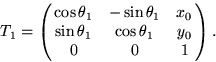
We are now prepared to determine the location of each link. The
position and orientation of link ![]() is determined by applying the
2D homogeneous transform matrix (2.10),
is determined by applying the
2D homogeneous transform matrix (2.10),
As shown in Figure 2.8, let ai-1 be the distance
between the joints in ![]() . The orientation difference between
. The orientation difference between
![]() and
and ![]() is denoted by the angle
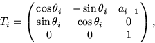
is denoted by the angle ![]() . Let Ti
represent a
. Let Ti
represent a ![]() homogeneous transform matrix
(2.10), specialized for link
homogeneous transform matrix
(2.10), specialized for link ![]() for
for ![]() ,in which
,in which
 |
(12) |
 |
(13) |
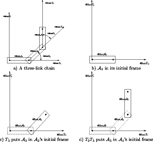
To gain an intuitive understanding of these transformations, consider
determining the configuration for link ![]() , as shown in
Figure 2.9. Figure 2.9.a shows a three-link
chain, in which
, as shown in
Figure 2.9. Figure 2.9.a shows a three-link
chain, in which ![]() is at its initial configuration, and the other
links are each offset by
is at its initial configuration, and the other
links are each offset by ![]() from the previous link.
Figure 2.9.b shows the frame in which the model for
from the previous link.
Figure 2.9.b shows the frame in which the model for
![]() is initially defined. The application of T3 causes a
rotation of
is initially defined. The application of T3 causes a
rotation of ![]() and a translation by a2. As shown in Figure
2.9.c, this places
and a translation by a2. As shown in Figure
2.9.c, this places ![]() in its appropriate configuration. Note
that
in its appropriate configuration. Note
that ![]() can be placed in its initial configuration, and it will be
attached correctly to
can be placed in its initial configuration, and it will be
attached correctly to ![]() . The application of T2 to the
previous result places both
. The application of T2 to the
previous result places both ![]() and
and ![]() in their proper
configurations, and
in their proper
configurations, and ![]() can be placed in its initial configuration.
can be placed in its initial configuration.
 |
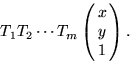
For revolute joints, the parameters ai are treated as constants,
and the ![]() are variables. The transformed mth link is
represented as
are variables. The transformed mth link is
represented as ![]() . In some
cases, the first link might have a fixed location in the world. In
this case, the revolute joints account for all degrees of freedom,
yielding
. In some
cases, the first link might have a fixed location in the world. In
this case, the revolute joints account for all degrees of freedom,
yielding ![]() . For prismatic joints, the
ai are treated as variables, as opposed to the
. For prismatic joints, the
ai are treated as variables, as opposed to the ![]() . Of
course, it is possible to include both types of joints in a single
kinematic chain.
. Of
course, it is possible to include both types of joints in a single
kinematic chain.